Douglas Blumeyer's RTT How-To
(to be broken out to pages named "Douglas Blumeyer's RTT How-To")
This is the reference I wish I had when I was learning RTT, or Regular Temperament Theory. There are other great resources out there, but this is how I would have liked to have learned it myself. I might say these materials lean more visual and geometric than others I've seen, and focus on elementary computation and representation rather than theory. It's not really a big picture introduction, it doesn't explore musical applications, and its algorithms are for humans, not computers. In any case, I hope others are able to benefit from these tools and explanations.
intro
What’s tempering, you ask, and why temper? I won’t be answering those questions in depth here. Plenty has been said about the “what” and “why” elsewhere[1]. These materials are about the “how”.
But I will at least give brief answers. In the most typical case, tempering means adjusting the tuning of the primes — the harmonic building blocks of your music — only a little bit, so that you can still sense what chords and melodies are “supposed” to be, but in just such a way that the interval math “adds up” in more practical ways than it does in pure just intonation (JI). This is also what equal divisions (EDs) do, but where EDs go “all the way”, compromising more JI accuracy for more ease of use, RTT finds a “middle path”: minimizing the accuracies you sacrifice, while maximizing ease of use. Understanding that much of the “what”, you can refer to this table to see basically “why”:
| ED | RTT (middle path) | JI | |
|---|---|---|---|
| ease of use | ★★★★ | ★★★ | ★ |
| harmonic accuracy | ★ | ★★★ | ★★★★ |
The point is that a tempered tuning manages to score high for both usability and harmonic accuracy, and therefore the case can be made that it is better overall than either a straight ED or straight JI. On this table (which reflects my opinion), RTT got six total stars while ED and JI each only got five. (And this doesn't even account for the power RTT has to create fascinating new harmonic effects, like comma pumps and essentially tempered chords, which EDs can do to a lesser extent.)
But, you protest: this tutorial is pretty long, and it contains a bunch of gnarly diagrams and advanced math concepts, so how could RTT possibly be easier to use than JI? Well, what I’ve rated above is the ease of use after you’ve chosen your particular ED, RTT, or JI tuning. It’s the ease of writing, reading, reasoning about, communicating about, teaching, performing, listening to, and analyzing the music in said tuning. This is different from how simple it is to determine a desirable tuning up front.
Determining desirable tunings is a whole other beast. Perhaps contrary to popular belief, xenharmonic musicians — composers and performers alike — can mostly insulate themselves from this stuff if they like. It’s fine to nab a popular and well-reviewed tuning off the shelf, without deeply understanding how or why it’s there, and just pump, jam, or riff away. There's a good chance you could naturally pick up what's cool about a tuning without ever learning the definition of "temper out" or "generator". But if you do want to be deliberate about it, to mod something, rifle through the obscure section, or even discover your own tuning, then you must prepare to delve deeper into the xenharmonic fold. That’s why this resource is here, for RTT.
As for whether determining a middle path tuning is any harder than determining an ED or JI tuning, I think it would be fair to say that in the exact same way that a middle path tuning — once attained — combines the strengths of ED and of JI, determining a middle path tuning combines the challenges of determining good ED tunings and of determining good JI tunings. You have been warned.
maps
In this first section, you will learn about maps — one of the basic building blocks of temperaments — and the effect maps have on musical intervals.
vectors and covectors
It’s hard to get too far with RTT before you understand vectors and covectors, so let’s start there.
Until stated otherwise, this material will assume the 5 prime-limit.
If you’ve previously worked with JI, you may already be familiar with vectors. Vectors are a compact way to express JI intervals in terms of their prime factorization, or in other words, their harmonic building blocks. In JI, and in most contexts in RTT, vectors simply list the count of each prime, in order. For example, 16/15 is [4 -1 -1⟩ because it has four 2’s in its numerator, one 3 in its denominator, and also one 5 in its denominator. You can look at each term as an exponent: 2⁴ × 3⁻¹ × 5⁻¹ = 16/15.
And if you’ve previously worked with EDOs, you may already be familiar with covectors. Covectors are a compact way to express EDOs in terms of the count of its steps it takes to reach its approximation of each prime harmonic, in order. For example, 12-EDO is ⟨12 19 28]. The first term is the same as the name of the EDO, because the first prime harmonic is 2/1, or in other words: the octave. So this covector tells us that it takes 12 steps to reach 2/1 (the octave), 19 steps to reach 3/1 (the tritave), and 28 steps to each 5/1 (the pentave). Any or all of those intervals may be approximate.
If the musical structure that the mathematical structure called a vector represents is an interval, the musical structure that the mathematical structure called a covector represents is called a map.
Note the different direction of the brackets between covectors and vectors: covectors ⟨] point left, vectors [⟩ point right.
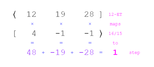
Covectors and vectors give us a way to bridge JI and EDOs. If the vector gives us a list of primes in a JI interval, and the covector tells us how many steps it takes to reach the approximation of each of those primes individually in an EDO, then when we put them together, we can see what step of the EDO should give the closest approximation of that JI interval. We say that the JI interval maps to that number of steps in the EDO. Calculating this looks like ⟨12 19 28][4 -1 -1⟩, and all that means is to multiply matching terms and sum the results (this is called the dot product).
So, 16/15 maps to one step in 12-EDO (see Figure 2a).
For another example, can quickly find the fifth size for 12-EDO from its map, because 3/2 is [-1 1 0⟩, and so ⟨12 19 28][-1 1 0⟩ = (12 × -1) + (19 × 1) = 7. Similarly, the major third — 5/4, or [-2 0 1⟩ — is simply 28 - 12 - 12 = 4.
WolframAlpha's syntax is slightly different than what we use in RTT, but it's pretty alright for a free online tool capable of handling most of the math we need to do in RTT, so we're going to be supplementing several topics with WolframAlpha examples as we go. Here's the first:
| input | output |
|---|---|
{12,19,28}.{-1,1,0}
|
7 |
tempering out commas
Here’s where things start to get really interesting.
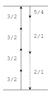
We can also see that the JI interval 81/80 maps to zero steps in 12-EDO, because ⟨12 19 28][-4 4 -1⟩ = 0; we therefore say this JI interval vanishes in 12-EDO, or that it is tempered out. This type of JI interval is called a comma, and this particular one is called the meantone comma.
The immediate conclusion is that 12-EDO is not equipped to approximate the meantone comma directly as a melodic or harmonic interval, and this shouldn’t be surprising because 81/80 is only around 20¢, while the (smallest) step in 12-EDO is five times that.
But a more interesting way to think about this result involves treating [-4 4 -1⟩ not as a single interval, but as the end result of moving by a combination of intervals. For example, moving up four fifths, 4 × [-1 1 0⟩ = [-4 4 0⟩, and then moving down one pentave [0 0 -1⟩, gets you right back where you started in 12-EDO. Or, in other words, moving by one pentave is the same thing as moving by four fifths (see Figure 2b). One can make compelling music that exploits such harmonic mechanisms.
From this perspective, the disappearance of 81/80 is not a shortcoming, but a fascinating feature of 12-EDO; we say that 12-EDO supports the meantone temperament. And 81/80 in 12-EDO is only the beginning of that journey. For many people, tempering commas is one of the biggest draws to RTT.
But we’re still only talking about JI and EDOs. If you’re familiar with meantone as a historical temperament, you may be aware already that it is neither JI nor an EDO. Well, we’ve got a ways to go yet before we get there.
One thing we can easily begin to do now, though, is this: refer to EDOs instead as ETs, or equal temperaments. The two terms are roughly synonymous, but have different implications and connotations. To put it briefly, the difference can be found in the names: 12 Equal Divisions of the Octave suggests only that your goal is equally dividing the octave, while 12 Equal Temperament suggests that your goal is to temper and that you have settled on a single equal step to accomplish that. Because we’re learning about temperament theory here, it would be more appropriate and accurate to use the local terminology. 12-ET it is, then.
approximating JI
If you’ve seen one map before, it’s probably ⟨12 19 28]. That’s because this map is the foundation of conventional Western tuning: 12 equal temperament. A major reason it stuck is because — for its low complexity — it can closely approximate all three of the 5 prime-limit harmonics 2, 3, and 5 at the same time.
One way to think of this is that 12:19:28 is an excellent low integer approximation of log(2:3:5). That's a really compact way of saying that each of these sets of three numbers has the same ratio between each pair of them:
- [math]\displaystyle{ \frac{19}{12} = 1.583 ≈ \frac{log(3)}{log(2)} = 1.585 }[/math]
- [math]\displaystyle{ \frac{28}{12} = 2.333 ≈ \frac{log(5)}{log(2)} = 2.322 }[/math]
- [math]\displaystyle{ \frac{28}{19} = 1.474 ≈ \frac{log(5)}{log(3)} = 1.465 }[/math]
You may be more familiar with seeing the base specified for a logarithm, but in this case the base is irrelevant as long as you use the same base for both numbers. If you don't see why, try experimenting with different bases and see that the ratio comes out the same[2].
But why take the logarithm at all? Because a) 2, 3, and 5 are not exponents, b) 12, 19, and 28 are exponents, and c) logarithms give exponents.
- 2, 3, and 5 are not exponents. They’re multipliers. To be specific, they’re multipliers of frequency. If the root pitch 1(/1) is 440Hz, then 2(/1) is 880Hz, 3(/1) is 1320Hz, and 5(/1) is 2200Hz.
- 12, 19, and 28 are exponents. Think of it this way: the map tells us to find some shared number g, called a generator, such that g¹² ≈ 2, g¹⁹ ≈ 3, and g²⁸ ≈ 5. It doesn’t tell us whether all of those approximations can be good at the same time, but it tells us that’s what we’re aiming for. For this map, it happens to be the case that a generator of around 1.059 will be best. Note that this generator is the same thing as one step of our ET. Also note that by thinking this way, we are thinking in terms of frequency (e.g. in Hz), not pitch (e.g. in cents): when we move repeatedly in pitch, we repeatedly add, which can be expressed as multiplication, e.g. 100¢ + 100¢ + 100¢ + 100¢ + 100¢ + 100¢ + 100¢ + 100¢ + 100¢ + 100¢ + 100¢ + 100¢ = 12×100¢ = 1200¢, while when we move repeatedly in frequency, we repeatedly multiply, which can be expressed as exponentiation, e.g. 1.059 × 1.059 × 1.059 × 1.059 × 1.059 × 1.059 × 1.059 × 1.059 × 1.059 × 1.059 × 1.059 × 1.059 = 1.059¹² ≈ 2. We can therefore say that frequency and pitch are two realms separated by one logarithmic order.
- logarithms give exponents. A logarithm answers the question, “What exponent do I raise this base to in order to get this value?” So when I say 12 = logg2 I’m saying there’s some base g which to the twelfth power gives 2, and when I say 19 = logg3 I’m saying there’s some base g which to the nineteenth power gives 3, etc. (That’s how I found 1.059, by the way; if g¹² ≈ 2, and I take the twelfth root of both sides, I get g = ¹²√2 ≈ 1.05946, and I could have just easily taken ¹⁹√3 ≈ 1.05952 or ²⁸√5 ≈ 1.05916).
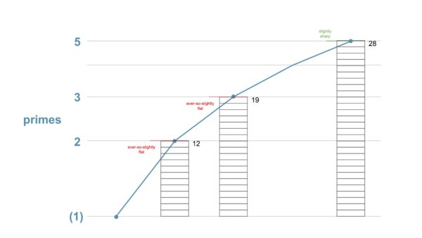
So when I say 12:19:28 ≈ log(2:3:5) what I’m saying is that there is indeed some shared generator g for which logg2 ≈ 12, logg3 ≈ 19, and logg5 ≈ 28 are all good approximations all at the same time, or, equivalently, a shared generator g for which g¹² ≈ 2, g¹⁹ ≈ 3, and g²⁸ ≈ 5 are all good approximations at the same time (see Figure 2c). And that’s a pretty cool thing to find! To be clear, with g = 1.059, we get g¹² ≈ 1.9982, g¹⁹ ≈ 2.9923, and g²⁸ ≈ 5.0291.
Another glowing example is the map ⟨53 84 123], for which a good generator will give you g⁵³ ≈ 2.0002, g⁸⁴ ≈ 3.0005, g¹²³ ≈ 4.9974. This speaks to historical attention given to 53-ET. So while 53:84:123 is an even better approximation of log(2:3:5) (and you won’t find a better one until 118:187:274), of course its integers aren’t as low, so that lessens its appeal.
Why is this rare? Well, it’s like a game of trying to get these numbers to line up (see Figure 2d):
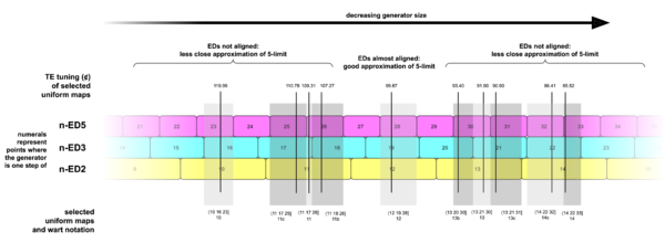
If the distance between entries in the row for 2 are defined as 1 unit apart, then the distance between entries in the row for prime 3 are 1/log₂3 units apart, and 1/log₂5 units apart for the prime 5. So, near-linings up don’t happen all that often![3] (By the way, any vertical line drawn through a chart like this is what we'll be calling here a uniform map; elsewhere you may find this called a “generalized patent val”.[4])
And why is this cool? Well, if ⟨12 19 28] approximates the harmonic building blocks well individually, then JI intervals built out of them, like 16/15, 5/4, 10/9, etc. should also be reasonably closely approximated overall, and thus recognizable as their JI counterparts in musical context. You could think of it like taking all the primes in a prime factorization and swapping in their approximations. For example, if 16/15 = 2⁴ × 3⁻¹ × 5⁻¹ ≈ 1.067, and ⟨12 19 28] approximates 2, 3, and 5 by 1.059¹² ≈ 1.998, 1.059¹⁹ ≈ 2.992, and 1.059²⁸ ≈ 5.029, respectively, then ⟨12 19 28] maps 16/15 to 1.998⁴ × 2.992⁻¹ × 5.029⁻¹ ≈ 1.059, which is indeed pretty close to 1.067. Of course, we should also note that 1.059 is the same as our step of ⟨12 19 28], which checks out with our calculation we made in the previous section that the best approximation of 16/15 in ⟨12 19 28] would be 1 step.
tuning & pure octaves
Now, because the octave is the interval of equivalence in terms of human pitch perception, it’s a major convenience to enforce pure octaves, and so many people prefer the first term to be exact. In fact, I’ll bet many readers have never even heard of or imagined impure octaves, if my own anecdotal experience is any indicator; the idea that I could temper octaves to optimize tunings came rather late to me.
Well, you’ll notice that in the previous section, we did approximate the octave, using 1.998 instead of 2. But another thing ⟨12 19 28] has going for it is that it excels at approximating 5-limit JI even if we constrain ourselves to pure octaves, locking g¹² to exactly 2: (¹²√2)¹⁹ ≈ 2.997 and (¹²√2)²⁸ ≈ 5.040. You can see that actually the approximation of 3 is even better here, marginally; it’s the error on 5 which is lamentable.
When we don’t enforce pure octaves, tuning becomes a more interesting problem. Approximating all three primes at once with the same generator is a balancing act. At least one of the primes will be tuned a bit sharp while at least one of them will be tuned a bit flat. In the case of ⟨12 19 28], the 5 is a bit sharp, and the 2 and 3 are each a tiny bit flat (as you can see in Figure 2c).
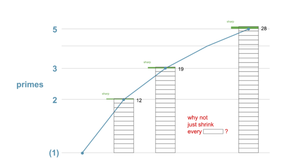
If you think about it, you would never want to tune all the primes sharp at the same time, or all of them flat; if you care about this particular proportion of their tunings, why wouldn’t you shift them all in the same direction, toward accuracy, while maintaining that proportion? (see Figure 2e)
This matter of choosing the exact generator for a map is called tuning, and if you’ll believe it, we won’t actually talk about that in detail again until much later. Temperament — the second ‘T’ in “RTT” — is the discipline concerned with choosing an interesting map, and tuning can remain largely independent from it. The temperament is only concerned with the fact that — no matter what exact size you ultimately make the generator — it is the case e.g. that 12 of them make a 2, 19 of them make a 3, and 28 of them make a 5. So, for now, whenever we show a value for g, assume we’ve given a computer a formula for optimizing the tuning to approximate all three primes equally well. As for us humans, let’s stay focused on tempering.
a multitude of maps
Suppose we want to experiment with ⟨12 19 28]’s map a bit. We’ll change one of the terms by 1, so now we have ⟨12 20 28]. Because the previous map did such a great job of approximating the 5-limit (i.e. log(2:3:5)), though, it should be unsurprising that this new map cannot achieve that feat. The proportions, 12:20:28, should now be about as out of whack as they can get. The best generator we can do here is about 1.0583 (getting a little more precise now), and 1.0583¹² ≈ 1.9738 which isn’t so bad, but 1.0583¹⁹ = 3.1058 and 1.0583²⁸ = 4.8870 which are both way off! And they’re way off in the opposite direction — 3.1058 is too big and 4.8870 is too small — which is why our tuning formula for g, which is designed to make the approximation good for every prime at once, can’t improve the situation: either sharpening or flattening helps one but hurts the other.
The results of such inaccurate approximation are a bit chaotic. A ratio like 16/15 — where the factors of 3 and 5 are on the same side of the fraction bar and therefore cancel out each other’s error — fares relatively alright, if by “alright” we mean it gets tempered out despite being about 112¢ in JI. On the other hand, an interval like 27/25 where the factors of 3 and 5 are on opposite sides of the fraction bar and thus their errors compound, gets mapped to a whopping 4 steps, despite only being about 133¢ in JI.
If your goal is to evoke JI-like harmony, then, ⟨12 20 28] is not your friend. Feel free to work out some other variations on ⟨12 19 28] if you like, such as ⟨12 19 29] maybe, but I guarantee you won’t find a better one that starts with 12 than ⟨12 19 28].
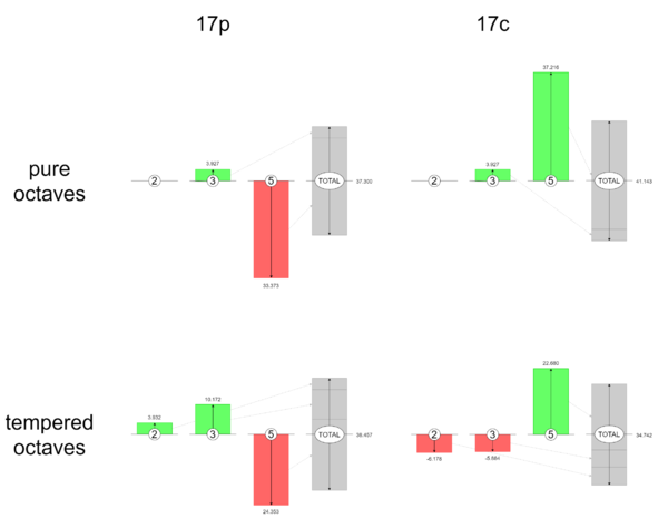
So the case is cut-and-dry for ⟨12 19 28], and therefore from now on I'm simply going to refer to this ET by "12-ET" rather than spelling out its map. But other ETs find themselves in trickier situations. Consider 17-ET. One option we have is the map ⟨17 27 39], with a generator of about 1.0418, and prime approximations of 2.0045, 3.0177, 4.9302. But we have a second reasonable option here, too, where ⟨17 27 40] gives us a generator of 1.0414, and prime approximations of 1.9929, 2.9898, and 5.0659. In either case, the approximations of 2 and 3 are close, but the approximation of 5 is way off. For ⟨17 27 39], it’s way small, while for ⟨17 27 40] it’s way big. The conundrum could be described like this: any generator we could find that divides 2 into about 17 equal steps can do a good job dividing 3 into about 27 equal steps, too, but it will not do a good job of dividing 5 into equal steps; 5 is going to land, unfortunately, right about in the middle between the 39th and 40th steps, as far as possible from either of these two nearest approximations. To do a good job approximating prime 5, we’d really just want to subdivide each of these steps in half, or in other words, we’d want 34-ET.
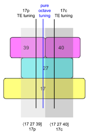
Curiously, ⟨17 27 39] is the map for which each prime individually is as closely approximated as possible when prime 2 is exact, so it is in a sense the naively best map for 17-ET, however, if that constraint is lifted, and we’re allowed to either temper prime 2 and/or choose the next-closest approximations for prime 5, the overall approximation can be improved; in other words, even though 39 steps can take you just a tiny bit closer to prime 5 than 40 steps can, the tiny amount by which it is closer is less than the improvements to the tuning of primes 2 and 3 you can get by using ⟨17 27 40]. So again, the choice is not always cut-and-dry; there’s still a lot of personal preference going on in the tempering process.
So some musicians may conclude “17-ET is clearly not cut out for 5-limit music,” and move on to another ET. Other musicians may snicker maniacally, and choose one or the other map, and begin exploiting the profound and unusual 5-limit harmonic mechanisms it affords. ⟨17 27 40], like ⟨12 19 28], tempers out the meantone comma [-4 4 -1⟩, so even though fifths and major thirds are different sizes in these two ETs, the relationship that four fifths equals one major third is shared. ⟨17 27 39], on the other hand, does not work like that, but what it does do is temper out 25/24, [-3 -1 2⟩, or in other words, it equates one fifth with two major thirds.
If you’re enforcing pure octaves, the difference between ⟨17 27 39] and ⟨17 27 40] is nominal, or contextual. The steps in either case are identical: exactly ¹⁷√2, or 1200/17=70.588¢. You simply choose to think of 5 as being approximated by either 39 or 40 of those steps, or imply it in your composition. But when octaves are freed to temper, then the difference between these two maps becomes pronounced. When optimizing for ⟨17 27 39], the best step size is 70.225¢, but when optimizing for ⟨17 27 40], the best step size is more like 70.820¢.
You will sometimes see maps like 17-ET’s distinguished from each other using names like 17p and 17c. This is called wart notation.
At this point you should have a pretty good sense for why choosing a map makes an important impact on how your music sounds. Now we just need to help you find and compare maps! Or, similarly, how to find and compare intervals to temper. To do this, we need to give you the ability to navigate tuning space.
projective tuning space
In this section, we will be going into potentially excruciating detail about how to read the projective tuning space diagram featured prominently in Paul Erlich's Middle Path paper. For me personally, attaining total understanding of this diagram was critical before the linear algebra stuff (that we'll discuss afterwards) started to mean much to me. But other people might not work that way, and the extent of detail I go into in this section is not necessary to become competent with RTT (in fact, to my delight, one of the points I make in this section was news to Paul himself). So if you're already confident about reading the PTS diagram, you may try skipping ahead.
intro to PTS

This is 5-limit projective tuning space, or PTS for short (see Figure 3a). This diagram was created by RTT pioneer Paul Erlich. It compresses a huge amount of valuable information into a small space. If at first it looks overwhelming or insane, do not despair. It may not be instantly easy to understand, but once you learn the tricks for navigating it from these materials, you will find it is very powerful. Perhaps you will even find patterns in it which others haven’t found yet.
I suggest you open this diagram in another window and keep it open as you proceed through these next few sections, as we will be referring to it frequently.
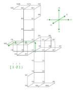
If you’ve worked with 5-limit JI before, you’re probably aware that it is three-dimensional. You’ve probably reasoned about it as a 3D lattice, where one axis is for the factors of prime 2, one axis is for the factors of prime 3, and one axis is for the factors of prime 5. This way, you can use vectors, such as [-4 4 -1⟩ or [1 -2 1⟩, just like coordinates.
PTS can be thought of as a projection of 5-limit JI map space, which similarly has one axis each for 2, 3, and 5. But it is no JI pitch lattice. In fact, in a sense, it is the opposite! This is because the coordinates in map space aren’t prime count lists, but maps, such as ⟨12 19 28]. That particular map is seen here as the biggish, slightly tilted numeral 12 just to the left of the center point.
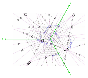
And the two 17-ETs we looked at can be found here too. ⟨17 27 40] is the slightly smaller numeral 17 found on the line labeled “meantone” which the 12 is also on, thus representing the fact we mentioned earlier that they both temper it out. The other 17, ⟨17 27 39], is found on the other side of the center point, aligned horizontally with the first 17. So you could say that map space plots ETs, showing how they are related to each other.
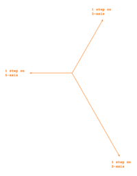
Of course, PTS looks nothing like this JI lattice (see Figure 3b). This diagram has a ton more information, and as such, Paul needed to get creative about how to structure it. It’s a little tricky, but we’ll get there. For starters, the axes are not actually shown on the PTS diagram; if they were, they would look like this (see Figure 3c).
The 2-axis points toward the bottom right, the 3-axis toward the top right, and the 5-axis toward the left. These are the positive halves of each of these axes; we don’t need to worry about the negative halves of any of them, because every term of every ET map is positive.
And so it makes sense that ⟨17 27 40] and ⟨17 27 39] are aligned horizontally, because the only difference between their maps is in the 5-term, and the 5-axis is horizontal.
scaled axes
You might guess that to arrive at that tilted numeral 12, you would start at the origin in the center, move 12 steps toward the bottom right (along the 2-axis), 19 steps toward the top right (not along, but parallel to the 3-axis), and then 28 steps toward the left (parallel to the 5-axis). And if you guessed this, you’d probably also figure that you could perform these moves in any order, because you’d arrive at the same ending position regardless (see Figure 3d).
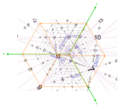
If you did guess this, you are on the right track, but the full truth is a bit more complicated than that.
The first difference to understand is that each axis’s steps have been scaled proportionally according to their prime (see Figure 3e). To illustrate this, let’s highlight an example ET and compare its position with the positions of three other ETs:
- the one which is one step away from it on the 5-axis,
- the one which is one step away from it on the 3-axis, and
- the one which is one step away from it on the 2-axis.
Our example ET will be 40. We'll start out at the map ⟨40 63 93]. This map is a default of sorts for 40-ET, because it’s the map where all three terms are as close as possible to JI when prime 2 is exact (we'll be calling it a simple map here, though elsewhere you may find it called a "patent val"[5]).
From here, let’s move by a single step on the 5-axis by adding 1 to the 5-term of our map, from 93 to 94, therefore moving to the map ⟨40 63 94]. This map is found directly to the left. This makes sense because the orientation of the 5-axis is horizontal, and the positive direction points out from the origin toward the left, so increases to the 5-term move us in that direction.
Back from our starting point, let’s move by a single step again, but this time on the 3-axis, by adding 1 to the 3-term of our map, from 63 to 64, therefore moving to the map ⟨40 64 93]. This map is found up and to the right. Again, this direction makes sense, because it’s the direction the 3-axis points.
Finally, let’s move by a single step on the 2-axis, from 40 to 41, moving to the map ⟨41 63 93], which unsurprisingly is in the direction the 2-axis points. This move actually takes us off the chart, way down here.
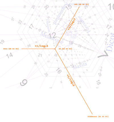
Now let’s observe the difference in distances (see Figure 3f). Notice how the distance between the maps separated by a change in 5-term is the smallest, the maps separated by a change in 3-term have the medium-sized distance, and maps separated by a change in the 2-term have the largest distance. This tells us that steps along the 3-axis are larger than steps along the 5-axis, and steps along the 2-axis are larger still. The relationship between these sizes is that the 3-axis step has been divided by the binary logarithm of 3, written log₂3, which is approximately 1.585, while the 5-axis step has been divided by the binary logarithm of 5, written log₂5, and which is approximately 2.322. The 2-axis step can also be thought of as having been divided by the binary logarithm of its prime, but because log₂2 is exactly 1, and dividing by 1 does nothing, the scaling has no effect on the 2-axis.
The reason Paul chose this particular scaling scheme is that it causes those ETs which are closer to JI to appear closer to the center of the diagram (and this is a useful property to organize ETs by). How does this work? Well, let’s look into it.
Remember that near-just ETs have maps whose terms are in close proportion to log(2:3:5). ET maps use only integers, so they can only approximate this ideal, but a theoretical pure JI map would be ⟨log₂2 log₂3 log₂5]. If we scaled this theoretical JI map by this scaling scheme, then, we’d get 1:1:1, because we’re just dividing things by themselves: log₂2/log₂2:log₂3/log₂3:log₂5/log₂5 = 1:1:1. This tells us that we should find this theoretical JI map at the point arrived at by moving exactly the same amount along the 2-axis, 3-axis, and 5-axis. Well, if we tried that, these three movements would cancel each other out: we’d draw an equilateral triangle and end up exactly where we started, at the origin, or in other words, at pure JI. Any other ET approximating but not exactly log(2:3:5) will be scaled to proportions not exactly 1:1:1, but approximately so, like maybe 1:0.999:1.002, and so you’ll move in something close to an equilateral triangle, but not exactly, and land in some interesting spot that’s not quite in the center. In other words, we scale the axes this way so that we can compare the maps not in absolute terms, but in terms of what direction and by how much they deviate from JI (see Figure 3g).
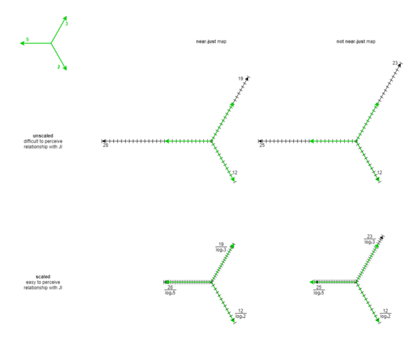
For example, let’s scale our 12-ET example:
- 12/log₂2 = 12
- 19/log₂3 ≈ 11.988
- 28/log₂5 ≈ 12.059
Clearly, 12:11.988:12.059 is quite close to 1:1:1. This checks out with our knowledge that it is close to JI, at least in the 5-limit.
But if instead we picked some random alternate mapping of 12-ET, like ⟨12 23 25], looking at those integer terms directly, it may not be obvious how close to JI this map is. However, upon scaling them:
- 12/log₂2 = 12
- 23/log₂3 ≈ 14.511
- 25/log₂5 ≈ 10.767
It becomes clear how far this map is from JI.
So what really matters here are the little differences between these numbers. Everything else cancels out. That 12-ET’s scaled 3-term, at ≈11.988, is ever-so-slightly less than 12, indicates that prime 3 is mapped ever-so-slightly flat. And that its 5-term, at ≈12.059, is slightly more than 12, indicates that prime 5 is mapped slightly sharp in 12. This checks out with the placement of 12 on the diagram: ever-so-slightly below and to the left of the horizontal midline, due to the flatness of the 3, and slightly further still to the left, due to the sharpness of the 5.
We can imagine that if we hadn’t scaled the steps, as in our initial naive guess, we’d have ended up nowhere near the center of the diagram. How could we have, if the steps are all the same size, but we’re moving 28 of them to the left, but only 12 and 19 of them to the bottom left and top right? We’d clearly end up way, way further to the left, and also above the horizontal midline. And this is where pretty much any near-just ET would get plotted, because 3 being bigger than 2 would dominate its behavior, and 5 being larger still than 3 would dominate its behavior.
perspective
The truth about distances between related ETs on the PTS diagram is actually slightly even more complicated than that, though; as we mentioned, the scaled axes are only the first difference from our initial guess. In addition to the effect of the scaling of the axes, there is another effect, which is like a perspective effect. Basically, as ETs get more complex, you can think of them as getting farther and farther away; to suggest this, they are printed smaller and smaller on the page, and the distances between them appear smaller and smaller too.
Remember that 5-limit JI is 3D, but we’re viewing it on a 2D page. It’s not the case that its axes are flat on the page. They’re not literally occupying the same plane, 120° apart from each other. That’s just not how axes typically work, and it’s not how they work here either! The 5-axis is perpendicular to the 2-axis and 3-axis just like typical Cartesian space. Again, we’re looking only at the positive coordinates, which is to say that this is only the +++ octant of space, which comes to a point at the origin (0,0,0) like the corner of a cube. So you should think of this diagram as showing that cubic octant sticking its corner straight out of the page at us, like a triangular pyramid. So we’re like a tiny little bug, situated right at the tip of that corner, pointing straight down the octant’s interior diagonal, or in other words the line equidistant from three axes, the line which we understand represents theoretically pure JI. So we see that in the center of the page, represented as a red hexagram, and then toward the edges of the page is our peripheral vision. (See Figure 3h.)
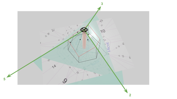
PTS doesn’t show the entire tuning cube. You can see evidence of this in the fact that some numerals have been cut off on its edges. We’ve cropped things around the central region of information, which is where the ETs best approximating JI are found (note how close 53-ET is to the center!). Paul added some concentric hexagons to the center of his diagram, which you could think of as concentric around that interior diagonal, or in other words, are defined by gradually increasing thresholds of deviations from JI for any one prime at a time.
No maps past 99-ET are drawn on this diagram. ETs with that many steps are considered too complex (read: big numbers, impractical) to bother cluttering the diagram with. Better to leave the more useful information easier to read.
Okay, but what about the perspective effect? Right. So every step further away on any axis, then, appears a bit smaller than the previous step, because it’s just a bit further away from us. And how much smaller? Well, the perspective effect is such that, as seen on this diagram, the distances between n-ETs are twice the size of the distances between 2n-ETs.
Moreover, there’s a special relationship between the positions of n-ETs and 2n-ETs, and indeed between n-ETs and 3n-ETs, 4n-ETs, etc. To understand why, it’s instructive to plot it out (see Figure 3i).
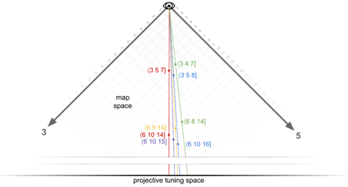
For simplicity, we’re looking at the octant cube here from the angle straight on to the 2-axis, so changes to the 2-terms don’t matter here. At the top is the origin; that’s the point at the center of PTS. Close-by, we can see the map ⟨3 5 7], and two closely related maps ⟨3 4 7] and ⟨3 5 8]. Colored lines have been drawn from the origin through these points to the black line in the top-right, which represents the page; this is portraying how if our eye is at that origin, where on the page these points would appear to be.
In between where the colored lines touch the maps themselves and the page, we see a cluster of more maps, each of which starts with 6. In other words, these maps are about twice as far away from us as the others. Let’s consider ⟨6 10 14] first. Notice that each of its terms is exactly 2x the corresponding term in ⟨3 5 7]. In effect, ⟨6 10 14] is redundant with ⟨3 5 7]. If you imagine doing a mapping calculation or two, you can easily convince yourself that you’ll get the same answer as if you’d just done it with ⟨3 5 7] instead and then simply divided by 2 one time at the end. It behaves in the exact same way as ⟨3 5 7] in terms of the relationships between the intervals it maps, the only difference being that it needlessly includes twice as many steps to do so, never using every other one. So we don’t really care about ⟨6 10 14]. Which is great, because it’s hidden exactly behind ⟨3 5 7] from where we’re looking.
The same is true of the map pair ⟨3 4 7] and ⟨6 8 14], as well as of ⟨3 5 8] and ⟨6 10 16]. Any map whose terms have a common divisor other than 1 is going to be redundant in this sense, and therefore hidden. You can imagine that even further past ⟨3 5 7] you’ll find ⟨9 15 21], ⟨12 20 28], and so on, and these are are called contorted maps[6]. More on those later. What’s important to realize here is that Paul found a way to collapse 3 dimensions worth of information down to 2 dimensions without losing anything important. Each of these lines connecting redundant ETs have been projected onto the page as a single point. That’s why the diagram is called "projective" tuning space.
Now, to find a 6-ET with anything new to bring to the table, we’ll need to find one whose terms don’t share a common factor. That’s not hard. We’ll just take one of the ones halfway between the ones we just looked at. How about ⟨6 11 14], which is halfway between ⟨6 10 14] and ⟨6 12 14]. Notice that the purple line that runs through it lands halfway between the red and blue lines on the page. Similarly, ⟨6 10 15] is halfway between ⟨6 10 14] and ⟨6 10 16], and its yellow line appears halfway between the red and green lines on the page. What this is demonstrating is that halfway between any pair of n-ETs on the diagram, whether this pair is separated along the 3-axis or 5-axis, you will find a 2n-ET. We can’t really demonstrate this with 3-ET and 6-ET on the diagram, because those ETs are too inaccurate; they’ve been cropped off. But if we return to our 40-ET example, that will work just fine.
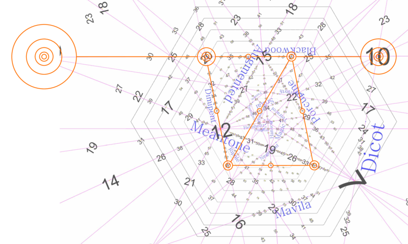
I’ve circled every 40-ET visible in the chart (see Figure 3j). And you can see that halfway between each one, there’s an 80-ET too. Well, sometimes it’s not actually printed on the diagram[7], but it’s still there. You will also notice that if we also land right about on top of 20-ET and 10-ET. That’s no coincidence! Hiding behind that 20-ET is a redundant 40-ET whose terms are all 2x the 20-ET’s terms, and hiding behind the 10-ET is a redundant 40-ET whose terms are all 4x the 40-ET’s terms (and also a redundant 20-ET and a 30-ET, and 50-ET, 60-ET, etc. etc. etc.)
Also, check out the spot halfway between our two 17-ETs: there’s the 34-ET we briefly mused about earlier, which would solve 17’s problem of approximating prime 5 by subdividing each of its steps in half. We can confirm now that this 34-ET does a superb job at approximating prime 5, because it is almost vertically aligned with the JI red hexagram.
Just as there are 2n-ETs halfway between n-ETs, there are 3n-ETs a third of the way between n-ETs. Look at these two 29-ETs here. The 58-ET is here halfway between them, and two 87-ETs are here each a third of the way between.
map space vs. tuning space
So far, we’ve been describing PTS as a projection of map space, which is to say that we’ve been thinking of maps as the coordinates. We should be aware that tuning space is a slightly different structure. In tuning space, coordinates are not maps, but tunings, specified in cents, octaves, or some other unit of pitch. So a coordinate might be ⟨6 10 14] in map space, but ⟨1200 2000 2800] in tuning space.
Both tuning space and map space project to the identical result as seen in Paul’s diagram, which is how we’ve been able to get away without distinguishing them thus far.
Why did I do this to you? Well, I decided map space was conceptually easier to introduce than tuning space. Paul himself prefers to think of this diagram as a projection of tuning space, however, so I don’t want to leave this material before clarifying the difference. Also, there are different helpful insights you can get from thinking of PTS as tuning space. Let’s consider those now.
The first key difference to notice is that we can normalize coordinates in tuning space, so that the first term of every coordinate is the same, namely, one octave, or 1200 cents. For example, note that while in map space, ⟨3 5 7] is located physically in front of ⟨6 10 14], in tuning space, these two points collapse to literally the same point, ⟨1200 2000 2800]. This can be helpful in a similar way to how the scaled axes of PTS help us visually compare maps’ proximity to the central JI spoke: they are now expressed closer to in terms of their deviation from JI, so we can more immediately compare maps to each other, as well as individually directly to the pure JI primes, as long as we memorize the cents values of those (they’re 1200, 1901.955, and 2786.314). For example, in map space, it may not be immediately obvious that ⟨6 9 14] is halfway between ⟨3 5 7] and ⟨3 4 7], but in tuning space it is immediately obvious that ⟨1200 1800 2800] is halfway between ⟨1200 2000 2800] and ⟨1200 1600 2800].
So if we take a look at a cross-section of projection again, but in terms of tuning space now (see Figure 3k), we can see how every point is about the same distance from us.
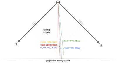
The other major difference is that tuning space is continuous, where map space is discrete. In other words, to find a map between ⟨6 10 14] and ⟨6 9 14], you’re subdividing it by 2 or 3 and picking a point in between, that sort of thing. But between ⟨1200 2000 2800] and ⟨1200 1800 2800] you’ve got an infinitude of choices smoothly transitioning between each other; you’ve basically got knobs you can turn on the proportions of the tuning of 2, 3, and 5. Everything from from ⟨1200 1999.999 2800] to ⟨1200 1901.955 2800] to ⟨1200 1817.643 2800] is along the way.
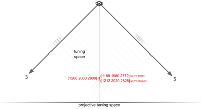
But perhaps even more interesting than this continuous tuning space that appears in PTS between points is the continuous tuning space that does not appear in PTS because it exists within each point, that is, exactly out from and deeper into the page at each point. In tuning space, as we’ve just established, there are no maps in front of or behind each other that get collapsed to a single point. But there are still many things that get collapsed to a single point like this, but in tuning space they are different tunings (see Figure 3l). For example, ⟨1200 1900 2800] is the way we’d write 12-ET in tuning space. But there are other tunings represented by this same point in PTS, such as ⟨1200.12 1900.19 2800.28] (note that in order to remain at the same point, we’ve maintained the exact proportions of all the prime tunings). That tuning might not be of particular interest. I just used it as a simple example to illustrate the point. A more useful example would be ⟨1198.440 1897.531 2796.361], which by some algorithm is the optimal tuning for 12-ET (minimizes error across primes or intervals); it may not be as obvious from looking at that one, but if you check the proportions of those terms with each other, you will find they are still exactly 12:19:28.
The key point here is that, as we mentioned before, the problems of tuning and tempering are largely separate. PTS projects all tunings of the same temperament to the same point. This way, issues of tuning are completely hidden and ignored on PTS, so we can focus instead on tempering.
regions
We’ve shown that ETs with the same number that are horizontally aligned differ in their mapping of 5, and ETs with the same number that are aligned on the 3-axis running bottom left to top right differ in their mapping of 3. These basic relationships can be extrapolated to be understood in a general sense. ETs found in the center-left map 5 relatively big and 2 and 3 relatively small. ETs found in the top-right map 3 relatively big and 2 and 5 relatively small. ETs found in the bottom-right map 2 relatively big and 3 and 5 relatively small. And for each of these three statements, the region on the opposite side maps things in the opposite way.
So: we now know which point is ⟨12 19 28], and we know a couple of 17’s, 40’s and a 41. But can we answer in the general case? Given an arbitrary map, like ⟨7 11 16], can we find it on the diagram? Well, you may look to the first term, 7, which tells you it’s 7-ET. There’s only one big 7 on this diagram, so it’s probably that. (You’re right). But that one’s easy. The 7 is huge.
What if I gave you ⟨43 68 100]. Where’s 43-ET? I’ll bet you’re still complaining: the map expresses the tempering of 2, 3, and 5 in terms of their shared generator, but doesn’t tell us directly which primes are sharp, and which primes are flat, so how could we know in which region to look for this ET?
The answer to that is, unfortunately: that’s just how it is. It can be a bit of a hunt sometimes. But the chances are, in the real world, if you’re looking for a map or thinking about it, then you probably already have at least some other information about it to help you find it, whether it’s memorized in your head, or you’re reading it off the results page for an automatic temperament search tool.
Probably you have the information about the primes’ tempering; maybe you get lucky and a 43 jumps out at you but it’s not the one you’re looking for, but you can use what you know about the perspectival scaling and axis directions and log-of-prime scaling to find other 43’s relative to it.
Or maybe you know which commas ⟨43 68 100] tempers out, so you can find it along the line for that comma’s temperament.
linear temperaments
We're about to take our first look at temperaments beyond mere equal temperaments. By the end of this section, you'll be able to explain the musical meaning of the patterns in the numerals along lines in PTS, the labels of these lines, as well as what's happening at their intersections and what their slopes mean. In other words, pretty much all of the major remaining visual elements on PTS should make sense to you.
temperament lines
So we understand the shape of projective tuning space. And we understand what points are in this space. But what about the magenta lines, now?
So far, we’ve only mentioned one of these lines: the one labelled “meantone”, noting that the fact that 12-ET and 17-ET appear on it means that either of them tempers out the meantone comma. In other words, this line represents the meantone temperament.
For another example, the line on the right side of the diagram running almost vertically which has the other 17-ET we looked at, as well as 10-ET and 7-ET, is labeled “dicot”, and so this line represents the dicot temperament, and unsurprisingly all of these ET’s temper out the dicot comma.
Simply put, lines on PTS are temperaments. Specifically, they are abstract regular temperaments. If you are a student of historical temperaments, you may be familiar with e.g. quarter-comma meantone; to an RTT practitioner, this is actually a specific tuning of the meantone temperament. Meantone is an abstract temperament, which encompasses a range of other possible temperaments and tunings.
If you’re new to RTT, all of the other temperaments besides meantone, like “dicot”, “porcupine”, and “mavila”, are probably unfamiliar and their names may seem sort of random or bizarre looking. Well, you’re not wrong about the names being random and bizarre. But mathematically and musically, these temperaments are every bit as much real and of interest as meantone. One day you too may compose a piece or write an academic paper about porcupine temperament.
But hold up now: points are ETs, which are temperaments, too, right? Well, yes, that’s still true. But while points are equal, or rank-1 temperaments, the lines represent what we call rank-2 temperaments. It may be helpful to differentiate the names in your mind in terms of their geometric dimensionality. Recall that projective tuning space has compressed all our information by one dimension; every point on our diagram is actually a line radiating out from our eye. So a rank-1 temperament is really a line, which is one-dimensional; rank-1, 1D. And the rank-2 temperaments, which are seen as lines in our diagram, are truly planes coming up out of the page, and planes are of course two-dimensional; rank-2, 2D. If you wanted to, you could even say 5-limit JI was a rank-3 temperament, because that’s this entire space, which is 3-dimensional; rank-3, 3D.
“Rank” has a slightly different meaning than dimension, but that’s not important yet. We’ll define rank, and discuss what exactly a rank-2 or -3 temperament means later. For now, it’s enough to know that each temperament line on this 5-limit PTS diagram is defined by tempering out a comma which has the same name. For now, we’re still focusing on visually how to navigate PTS. So the natural thing to wonder next, then, is what’s up with the slopes of all these temperament lines?
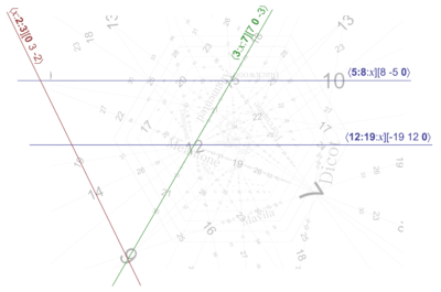
Let’s begin with a simple example: the perfectly horizontal line that runs through just about the middle of the page, through the numeral 12, labelled “compton”. What’s happening along this line? Well, as we know, moving to the left means tuning 5 sharper, and moving to the right means tuning 5 flatter. But what about 2 and 3? Well, they are changing as well: 2 is sharp in the bottom right, and 3 is sharp in the top right, so when we move exactly rightward, 2 and 3 are both getting sharper (though not as directly as 5 is getting flatter). But the critical thing to observe here is that 2 and 3 are sharpening at the exact same rate. Therefore the approximations of primes 2 and 3 are in a constant ratio with each other along horizontal lines like this. Said another way, if you look at the 2 and 3 terms for any ET’s map on this line, the ratio between its term for 2 and 3 will be identical.
Let’s grab some samples to confirm. We already know that 12-ET here looks like ⟨12 19] (I’m dropping the 5 term for now). The 24-ET here looks like ⟨24 38], which is simply 2×⟨12 19]. The 36-ET here looks like ⟨36 57] = 3×⟨12 19]. And so on. So that’s why we only see multiples of 12 along this line: because 12 and 19 are co-prime, so the only other maps which could have them in the same ratio would be multiples of them.
Let’s look at the other perfectly horizontal line on this diagram. It’s found about a quarter of the way down the diagram, and runs through the 10-ET and 20-ET we looked at earlier. This one’s called “blackwood”. Here, we can see that all of its ETs are all multiples of 5. In fact, 5-ET itself is on this line, though we can only see a sliver of its giant numeral off the left edge of the diagram. Again, all of its maps have locked ratios between their mappings of prime 2 and prime 3: ⟨5 8], ⟨10 16], ⟨15 24], ⟨20 32], ⟨40 64], ⟨80 128], etc. You get the idea.
So what do these two temperaments have in common such that their lines are parallel? Well, they’re defined by commas, so why don’t we compare their commas. The compton comma is [-19 12 0⟩, and the blackwood comma is [8 -5 0⟩[8]. What sticks out about these two commas is that they both have a 5-term of 0. This means that when we ask the question “how many steps does this comma map to in a given ET”, the ET’s mapping of 5 is irrelevant. Whether we check it in ⟨40 63 93] or ⟨40 63 94], the result is going to be the same. So if ⟨40 63 93] tempers out the blackwood comma, then ⟨40 63 94] also tempers out the blackwood comma. And if ⟨24 38 56] tempers out compton, then ⟨24 38 55] tempers out compton. And so on.
Similar temperaments can be found which include only 2 of the 3 primes at once. Take “augmented”, for instance, running from bottom-left to top-right. This temperament is aligned with the 3-axis. This tells us several equivalent things: that relative changes to the mapping of 3 are irrelevant for augmented temperament, that the augmented comma has no 3’s in its prime factorization, and the ratios of the mappings of 2 and 5 are the same for any ET along this line. Indeed we find that the augmented comma is [7 0 -3⟩, or 128/125, which has no 3’s. And if we sample a few maps along this line, we find ⟨12 19 28], ⟨9 14 21], ⟨15 24 35], ⟨21 33 48], ⟨27 43 63], etc., for which there is no pattern to the 3-term, but the 2- and 5-terms for each are in a 3:7 ratio.
There are even temperaments whose comma includes only 3’s and 5’s, such as “bug” temperament, which tempers out 27/25, or [0 3 -2⟩. If you look on this PTS diagram, however, you won’t find bug. Paul chose not to draw it. There are infinite temperaments possible here, so he had to set a threshold somewhere on which temperaments to show, and bug just didn’t make the cut in terms of how much it distorts harmony from JI. If he had drawn it, it would have been way out on the left edge of the diagram, completely outside the concentric hexagons. It would run parallel to the 2-axis, or from top-left to bottom-right, and it would connect the 5-ET (the huge numeral which is cut off the left edge of the diagram so that we can only see a sliver of it) to the 9-ET in the bottom left, running through the 19-ET and 14-ET in-between. Indeed, these ET maps — ⟨9 14 21], ⟨5 8 12], ⟨19 30 45], and ⟨14 22 33] — lock the ratio between their 3-terms and 5-terms, in this case to 2:3.
Those are the three simplest slopes to consider, i.e. the ones which are exactly parallel to the axes (see Figure 4a). But all the other temperament lines follow a similar principle. Their slopes are a manifestation of the prime factors in their defining comma. If having zero 5’s means you are perfectly horizontal, then having only one 5 means your slope will be close to horizontal, such as meantone [-4 4 -1⟩ or helmholtz [-15 8 1⟩. Similarly, magic [-10 -1 5⟩ and würschmidt [17 1 -8⟩, having only one 3 apiece, are close to parallel with the 3-axis, while porcupine [1 -5 3⟩ and ripple [-1 8 -5⟩, having only one 2 apiece, are close to parallel with the 2-axis.
Think of it like this: for meantone, a change to the mapping of 5 doesn’t make near as much of a difference to the outcome as does a change to the mapping of 2 or 3, therefore, changes along the 5-axis don’t have near as much of an effect on that line, so it ends up roughly parallel to it.
scale trees
Patterns, patterns, everywhere. PTS is chock full of them. One pattern we haven’t discussed yet is the pattern made by the ETs that fall along each temperament line.
Let’s consider meantone as our first example. Notice that between 12 and 7, the next-biggest numeral we find is 19, and 12+7=19. Notice in turn that between 12 and 19 the next-biggest numeral is 31, and 12+19=31, and also that between 19 and 7 the next-biggest numeral is 26, and 19+7=26. You can continue finding deeper ETs indefinitely following this pattern: 43 between 12 and 31, 50 between 31 and 19, 45 between 19 and 26, 33 between 26 and 7. In fact, if we step back a bit, remembering that the huge numeral just off the left edge is a 5, we can see that 12 is there in the first place because 5+7=12.
This effect is happening on every other temperament line. Look at dicot. 10+7=17. 10+17=27. 17+7=24. Etc.[9]
To fully understand why this is happening, we need a crash course in mediants, and the The Stern-Brocot tree.
The mediant of two fractions [math]\displaystyle{ \frac ab }[/math] and [math]\displaystyle{ \frac cd }[/math] is [math]\displaystyle{ \frac{a+c}{b+d} }[/math]. It’s sometimes called the freshman’s sum because it’s an easy mistake to make when first learning how to add fractions. And while this operation is certainly not equivalent to adding two fractions, it does turn out to have other important mathematical properties. The one we’re leveraging here is that the mediant of two numbers is always greater than one and less than the other. For example, the mediant of [math]\displaystyle{ \frac 35 }[/math] and [math]\displaystyle{ \frac 23 }[/math] is [math]\displaystyle{ \frac 58 }[/math], and it’s easy to see in decimal form that 0.625 is between 0.6 and 0.666.
The Stern-Brocot tree is a helpful visualization of all these mediant relations. Flanking the part of the tree we care about — which comes up in the closely-related theory of MOS scales, where it is often referred to as the “scale tree” — are the extreme fractions [math]\displaystyle{ \frac 01 }[/math] and [math]\displaystyle{ \frac 11 }[/math]. Taking the mediant of these two gives our first node: [math]\displaystyle{ \frac 12 }[/math]. Each new node on the tree drops an infinitely descending line of copies of itself on each new tier. Then, each node branches to either side, connecting itself to a new node which is the mediant of its two adjacent values. So [math]\displaystyle{ \frac 01 }[/math] and [math]\displaystyle{ \frac 12 }[/math] become [math]\displaystyle{ \frac 13 }[/math], and [math]\displaystyle{ \frac 12 }[/math] and [math]\displaystyle{ \frac 11 }[/math] become [math]\displaystyle{ \frac 23 }[/math]. In the next tier, [math]\displaystyle{ \frac 01 }[/math] and [math]\displaystyle{ \frac 13 }[/math] become [math]\displaystyle{ \frac 14 }[/math], [math]\displaystyle{ \frac 13 }[/math] and [math]\displaystyle{ \frac 12 }[/math] become [math]\displaystyle{ \frac 25 }[/math], [math]\displaystyle{ \frac 12 }[/math] and [math]\displaystyle{ \frac 23 }[/math] become [math]\displaystyle{ \frac 35 }[/math], and [math]\displaystyle{ \frac 23 }[/math] and [math]\displaystyle{ \frac 11 }[/math] become [math]\displaystyle{ \frac 34 }[/math].[10] The tree continues forever.
So what does this have to do with the patterns along the temperament lines in PTS? Well, each temperament line is kind of like its own section of the scale tree. The key insight here is that in terms of meantone temperament, there’s more to 7-ET than simply the number 7. The 7 is just a fraction’s denominator. The numerator in this case is 3. So imagine a [math]\displaystyle{ \frac 37 }[/math] floating on top of the 7-ET there. And there’s more to 5-ET than simply the number 5, in that case, the fraction is the [math]\displaystyle{ \frac 25 }[/math]. So the mediant of [math]\displaystyle{ \frac 25 }[/math] and [math]\displaystyle{ \frac 37 }[/math] is [math]\displaystyle{ \frac{5}{12} }[/math]. And if you compare the decimal values of these numbers, we have 0.4, 0.429, and 0.417. Success: [math]\displaystyle{ \frac{5}{12} }[/math] is between [math]\displaystyle{ \frac 25 }[/math] and [math]\displaystyle{ \frac 37 }[/math] on the meantone line. You may verify yourself that the mediant of [math]\displaystyle{ \frac{5}{12} }[/math] and [math]\displaystyle{ \frac 37 }[/math], [math]\displaystyle{ \frac{8}{19} }[/math], is between them in size, as well as [math]\displaystyle{ \frac{7}{17} }[/math] being between [math]\displaystyle{ \frac 25 }[/math] and [math]\displaystyle{ \frac{5}{12} }[/math] in size.
In fact, if you followed this value along the meantone line all the way from [math]\displaystyle{ \frac 25 }[/math] to [math]\displaystyle{ \frac 37 }[/math], it would vary continuously from 0.4 to 0.429; the ET points are the spots where the value happens to be rational.
Okay, so it’s easy to see how all this follows from here. But where the heck did I get [math]\displaystyle{ \frac 25 }[/math] and [math]\displaystyle{ \frac 37 }[/math] in the first place? I seemed to pull them out of thin air. And what the heck is this value?
generators
The answer to both of those questions is: it’s the generator (in this case, the meantone generator).
A generator is an interval which generates a temperament. Again, if you’re already familiar with MOS scales, this is the same concept. If not, all this means is that if you repeatedly move by this interval, you will visit the pitches you can include in your tuning.
We briefly looked at generators earlier. We saw how the generator for 12-ET was about 1.059, because repeated movement is like repeated multiplication (1.059 × 1.059 × 1.059 ...) and 1.059¹² ≈ 2, 1.059¹⁹ ≈ 3, and 1.059²⁸ ≈ 5. This meantone generator is the same basic idea, but there’s a couple of important differences we need to cover.
First of all, and this difference is superficial, it’s in a different format. We were expressing 12-ET’s generator 1.059 as a frequency multiplier; it’s like 2, 3, or 5, and this could be measured in Hz, say, by multiplying by 440 if A4 was our 1/1 (1.059 away from A is 466Hz, which is #A). But the meantone generators we’re looking at now in forms like [math]\displaystyle{ \frac 25 }[/math], [math]\displaystyle{ \frac 37 }[/math], or [math]\displaystyle{ \frac{5}{12} }[/math], are expressed as fractional octaves, i.e. they’re in terms of pitch, something that could be measured in cents if we multiplied by 1200 (2/5 × 1200¢ = 480¢). We have a special way of writing fractional octaves, and that’s with a backslash instead of a slash, like this: 2\5, 3\7, 5\12.
Cents and Hertz values can readily be converted between one form and the other, so it’s the second difference which is more important. It’s their size. If we do convert 12-ET’s generator to cents so we can compare it with meantone’s generator at 12-ET, we can see that 12-ET’s generator is 100¢ (log₂1.059 × 1200¢ = 100¢) while meantone’s generator at 12-ET is 500¢ (5/12 × 1200¢ = 500¢). What is the explanation for this difference?
Well, notice that meantone is not the only temperament which passes through 12-ET. Consider augmented temperament. Its generator at 12-ET is 400¢[11]. What's key here is that all three of these generators — 100¢, 500¢, and 400¢ — are multiples of 100¢.
Let’s put it this way. When we look at 12-ET in terms of itself, rather than in terms of any particular rank-2 temperament, its generator is 1\12. That’s the simplest, smallest generator which if we iterate it 12 times will touch every pitch in 12-ET. But when we look at 12-ET not as the end goal, but rather as a foundation upon which we could work with a given temperament, things change. We don’t necessarily need to include every pitch in 12-ET to realize a temperament it supports.
For example, for meantone, even if I iterated the generator only four times, starting at step 0, touching steps 5, 10, 3 (it would be 15, but we octave-reduce here, subtracting 12 to stay within 12, landing back at 15 - 12 = 3), and 8, we’d realize meantone. That’s because fourths and fifths are octave-complements, and so in a sense they are equivalent. So, moving four fourths up like this is the same thing as moving four fifths down, and we can see that gets me to the same place as if I moved one major third down, which — being 4 steps — would also take me to step 8. That's the central idea of meantone temperament, and so this is what I mean by we've "realized" it.
If we continued to iterate this 12-ET meantone generator, we would happen to eventually touch every pitch in 12-ET, because 5 and 12 are coprime; we’d continue onward from 8 to 1 (13 - 12 = 1), then 6, 11, 4, 9, 2, 7, and circle back to 0. On the other hand, augmented temperament in 12-ET could never reach most of the pitches, because 4 is not coprime with 12; the 4\12 generator is essentially 1\3, and can only reach 0, 4, and 8. From augmented temperament’s perspective, that’s acceptable, though: this set of pitches still realizes the fact that three major thirds get you back where you started, which is its whole point.
The fact that both the augmented and meantone temperament lines pass through 12-ET doesn’t mean that you need the entirety of 12-ET to play either one; it means something more like this: if you had an instrument locked into 12-ET, you could use it to play some kind of meantone and some kind of augmented. 12-ET is not necessarily the most interesting manifestation of either meantone or augmented; it’s merely the case that it technically supports either one. The most interesting manifestations of meantone or augmented may lay between ETs, and/or boast far more than 12 notes.
We mentioned that the generator value changes continuously as we move along a temperament line. So just to either side of 12-ET along the meantone line, the tuning of 2, 3, and 5 supports a generator size which in turn supports meantone, but it wouldn’t support augmented. And just to either side of 12-ET along the augmented line, the tuning of 2, 3, and 5 supports a generator which still supports augmented, but not meantone. 12-ET, we could say, is a convergence point between the meantone generator and the augmented generator. But it is not a convergence point because the two generators become identical in 12-ET, but rather because they can both be achieved in terms of 12-ET’s generator. In other words, 5\12 ≠ 4\12, but they are both multiples of 1\12.
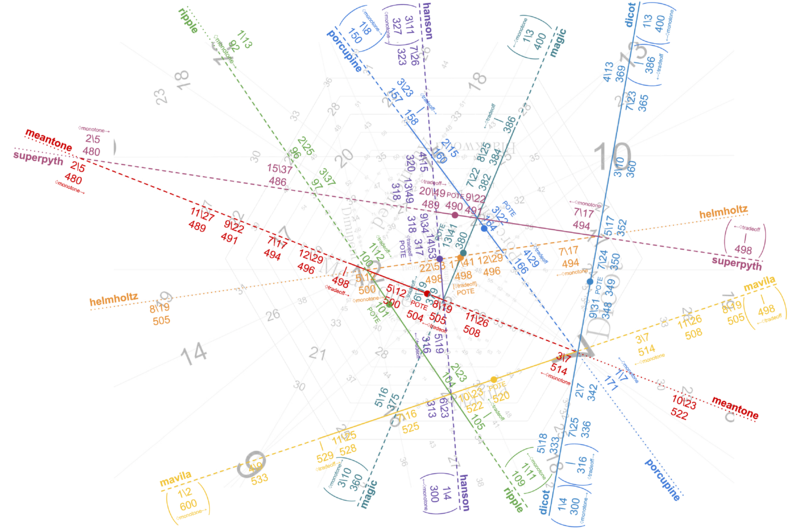
Here’s a diagram that shows how the generator size changes gradually across each line in PTS. It may seem weird how the same generator size appears in multiple different places across the space. But keep in mind that pretty much any generator is possible pretty much anywhere here. This is simply the generator size pattern you get when you lock the period to exactly 1200 cents, to establish a common basis for comparison. These are called linear temperaments. This is what enables us to produce maps of temperaments such as the one found at this Xen wiki page, or this chart here (see Figure 4b).
periods and generators
Earlier we mentioned the term “rank”. I warned you then that it wasn’t actually the same thing as dimensionality, even though we could use dimensionality in the PTS to help differentiate rank-2 from rank-1 temperaments. Now it’s time to learn the true meaning of rank: it’s how many generators a temperament has. So, it is the dimensionality of the tempered lattice; but it's still important to stay clear about the fact that it's different from the dimensionality of the original system from which you are tempering.
When we spoke of the generator for a rank-2 temperament such as meantone, we were taking advantage of the fact that the other generator is generally assumed to be the octave, and it gets its own special name: the period. It’s technically a generator too, but when we say “the” generator of a rank-2 temperament, we mean the one that’s not the period.
In rank-2 temperaments, the period usually serves as the interval of repetition. Rank-1 temperaments have only one generator, but by definition it’s some integer fraction of the interval of repetition. So, in an ET, the period is not literally a separate generator, but it may still make sense in context to refer to its interval of repetition — octave or otherwise — as the period, especially when comparing the ET with a related rank-2 temperament.
As we’ll soon see, there’s more than one way to generate a given rank-2 temperament. For example, meantone can be generated by an octave and a fourth. But it could equivalently be generated by an octave and a fifth. Or an octave and an augmented unison. It could even be generated by cycling a fourth against a fifth. And so on.
And so it’s good to have a standard form for the generators of a rank-2 temperament. One excellent standard is to set the period to an octave and the generator set to anything less than half the size of the period, as we did earlier, and again, when in this form, we call the temperament a linear temperament (not all rank-2 temperaments can be linear, e.g. if they repeat multiple times per octave, such as blackwood 5x or augmented 3x).
Let’s bring up MOS theory again. We mentioned earlier that you might have been familiar with the scale tree if you’d worked with MOS scales before, and if so, the connection was scale cardinalities, or in other words, how many notes are in the resultant scales when you continuously iterate the generator until you reach points where there are only two scale step sizes. At these points scales tend to sound relatively good, and this is in fact the definition of a MOS scale. There’s a mathematical explanation for how to know, given a ratio between the size of your generator and period, the cardinalities of scales possible; we won’t re-explain it here. The point is that the scale tree can show you that pattern visually. And so if each temperament line in PTS is its own segment of the scale tree, then we can use it in a similar way.
For example, if we pick a point along the meantone line between 46 and 29, the cardinalities will be 5, 12, 17, 29, 46, etc. If we chose exactly the point at 29, then the cardinality pattern would terminate there, or in other words, eventually we’ll hit a scale with 29 notes and instead of two different step sizes there would only be one, and there’s no place else to go from there. The system has circled back around to its starting point, so it’s a closed system. Further generator iterations will only retread notes you’ve already touched. The same would be true if you chose exactly the point at 46, except that’s where you’d hit an ET instead.
Between ETs, in the stretches of rank-2 temperament lines where the generator is not a rational fraction of the octave, theoretically those temperaments could have infinite pitches; you could continuously iterate the generator and you’d never exactly circle back to the point where you started. If bigger numbers were shown on PTS, you could continue to use those numbers to guide your cardinalities forever.
The structure when you stop iterating the meantone generator with five notes is called meantone[5]. If you were to use the entirety of 12-ET as meantone then that’d be meantone[12]. But you can also realize meantone[12] in 19-ET; in the former you have only one step size, but in the latter you have two. You can’t realize meantone[19] in 12-ET, but you could also realize it in 31-ET.
meet and join
We’ve seen how 12-ET is found at the convergence of meantone and augmented temperaments, and therefore supports both at the same time. In fact, no other ET can boast this feat. Therefore, we can even go so far as to describe 12-ET as the meeting of the meantone line and the augmented line. Using the pipe operator “|” to mean “meet”, then, we could call 12-ET “meantone|augmented”, read "meantone meet augmented". In other words, we express a rank-1 temperament in terms of two rank-2 temperaments.
For another rank-1 example, we could call 7-ET “meantone|dicot”, because it is the meeting of meantone and dicot temperaments.
We can conclude that there’s no “blackwood|compton” temperament, because those two lines are parallel. In other words, it’s impossible to temper out the blackwood comma and compton comma simultaneously. How could it ever be the case that 12 fifths take you back where you started yet also 5 fifths take you back where you started?[12]
Similarly, we can express rank-2 temperaments in terms of rank-1 temperaments. Have you ever heard the expression “two points make a line”? Well, if we choose two ETs from PTS, then there is one and only one line that runs through both of them. So, by choosing those ETs, we can be understood to be describing the rank-2 temperament along that line, or in other words, the one and only temperament whose comma both of those ETs temper out.
For example, we could choose 7-ET and 12-ET. Looking at either 12-ET or 7-ET, we can see that many, many temperament lines pass through them individually. Even more pass through them which Paul chose (via a complexity threshold) not to show. But there’s only one line which runs through both 7-ET and 12-ET, and that’s the meantone line. So of all the commas that 7-ET tempers out, and all the commas that 12-ET tempers out, there’s only a single one which they have in common, and that’s the meantone comma. Therefore we could give meantone temperament another name, and that’s “7&12”; in this case we use the ampersand operator, not the pipe. This operator is called "join", so we can read that "7 join 12".[13]
When specifying a rank-1 temperament in terms of two rank-2 temperaments, an obvious constraint is that the two rank-2 temperaments cannot be parallel. When specifying a rank-2 temperament in terms of two rank-1 temperaments, it seems like things should be more open-ended. Indeed, however, there is a special additional constraint on either method, and they’re related to each other. Let’s look at rank-2 as the join of rank-1 first.
7&12 is valid for meantone. So is 5&7, and 7&12. 12&19 and 19&7 are both fine too, and so are 5&17 and 17&12. Yes, these are all literally the same thing (though you may connote a meantone generator size on the meantone line somewhere between these two ETs). So how could we mess this one up, then? Well, here’s our first counterexamples: 5&19, 7&17, and 17&19. And what problem do all these share in common? The problem is that between 5 and 19 on the meantone line we find 12, and 12 is a smaller number than 19 (or, if you prefer, on PTS, it is printed as a larger numeral). It’s the same problem with 17&19, and with 7&17 the problem is that 12 is smaller than 17. It’s tricky, but you have to make sure that between the two ETs you join there’s not a smaller ET (which you should be joining instead). The reason why is out of scope to explain here, but we’ll get to it eventually.
I encourage you to spend some time playing around with Graham Breed's online RTT tool. For example, at http://x31eq.com/temper/net.html you can enter 12&19 in the "list of steps to the octave" field and 5 in the "limit" field and Submit, and you'll be taken to a results page for meantone.
And the related constraint for rank-1 from two rank-2 is that you can’t choose two temperaments whose names are printed smaller on the page than another temperament between them. More on that later.
matrices
From the PTS diagram, we can visually pick out rank-1 temperaments at the meetings of rank-2 temperaments as well as rank-2 temperaments as the joinings of rank-1 temperaments. But we can also understand these results through covectors and vectors. And we're going to need to learn how, because PTS can only take us so far. 5-limit PTS is good for humans because we live in a physically 3-dimensional world (and spend a lot of time sitting in front of 2D pages on paper and on computer screens), but as soon as you want to start working in 7-limit harmony, which is 4D, visual analogies will begin to fail us, and if we’re not equipped with the necessary mathematical abstractions, we’ll no longer be able to effectively navigate.
Don’t worry: we’re not going 4D just yet. We’ve still got plenty we can cover using only the 5-limit. But we may put away PTS for a couple sections. It’s matrix time. By the end of this section, you'll understand how to represent a temperament in matrix form, how to interpret them, notate them, and use them, as well as how to apply important transformations between different kinds of these matrices.
mapping-row bases and comma bases
19-ET. Its map is ⟨19 30 44]. We also now know that we could call it “meantone|magic”, because we find it at the meeting of the meantone and magic temperament lines. But how would we mathematically, non-visually make this connection?
The first critical step is to recall that temperaments are defined by commas, which can be expressed as vectors. So, we can represent meantone using the meantone comma, [-4 4 -1⟩, and magic using the magic comma [-10 -1 5⟩.
The meet of two vectors can be represented as a matrix. If a vector is like a list of numbers, a matrix is a table of them. Technically, vectors are vertical lists of numbers, or columns, so when we put meantone and magic together, we get a matrix that looks like this:
[math]\displaystyle{ \left[ \begin{array} {rrr} -4 & -10 \\ 4 & -1 \\ -1 & 5 \end{array} \right] }[/math]
We call such a matrix a comma basis. The plural of “basis” is “bases”, but pronounced like BAY-sees (/ˈbeɪ siz/).
Now how in the world could that matrix represent the same temperament as ⟨19 30 44]? Well, they’re two different ways of describing it. ⟨19 30 44], as we know, tells us how many generator steps it takes to reach each prime approximation. This matrix, it turns out, is an equivalent way of stating the same information. This matrix is a minimal representation of the null-space of that mapping, or in other words, of all the commas it tempers out. (Don't worry about the word "mapping" just yet; for now, just imagine I'm writing "map". We'll explain the difference very soon.).
This was a bit tricky for me to get my head around, so let me hammer this point home: when you say "the null-space", you're referring to the entire infinite set of all commas that a mapping tempers out, not only the two commas you see in any given basis for it. Think of the comma basis as one of many valid sets of instructions to find every possible comma, by adding or subtracting these two commas from each other[14]. The math term for adding and subtracting vectors like this, which you will certainly see plenty of as you explore RTT, is "linear combination". It should be visually clear from the PTS diagram that this 19-ET comma basis couldn't be listing every single comma 19-ET tempers out, because we can see there are at least four temperament lines that pass through it (there are actually infinity of them!). But so it turns out that picking two commas is perfectly enough; every other comma that 19-ET tempers out could be expressed in terms of these two!
Try one. How about the hanson comma, [6 5 -6⟩. Well that one’s too easy! Clearly if you go down by one magic comma to [10 1 -5⟩ and then up by one meantone comma you get one hanson comma. What you’re doing when you’re adding and subtracting multiples of commas from each other like this is technically called “Gauss-Jordan elimination”. Feel free to work through any other examples yourself.
A good way to explain why we don’t need three of these commas is that if you had three of them, you could use any two of them to create the third, and then subtract the result from the third, turning that comma into a zero vector, or a vector with only zeroes, which is pretty useless, so we could just discard it.
And a potentially helpful way to think about why any other interval arrived at through linear combinations of the commas in a basis would also be a valid column in the basis is this: any of these interval vectors, by definition, is mapped to zero steps by the mapping. So any combination of them will also map to zero steps, and thus be a comma that is tempered out by the temperament.
When written with the ⟨] notation, we’re expressing maps in “covector” form, or in other words, as the opposite of vectors. But we can also think of maps in terms of matrices. If vectors are like matrix columns, maps are like matrix rows. So while we have to write [-4 4 -1⟩ vertically when in matrix form, ⟨19 30 44] stays horizontal.
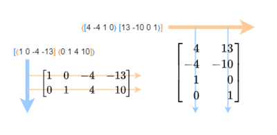
We can extend our angle bracket notation (technically called bra-ket notation, or Dirac notation[15]) to handle matrices by nesting rows inside columns, or columns inside rows (see Figure 5a). For example, we could have written our comma basis like this: ⟨[-4 4 -1⟩ [-10 -1 5⟩]. Starting from the outside, the ⟨] tells us to think in terms of a row. It's just that this covector isn't a covector of numbers, like the ones we've gotten used to by now, but rather a covector of columns of numbers. So this row houses two such columns. Alternatively, we could have written this same matrix like [⟨-4 -10] ⟨4 -1] ⟨-1 5]⟩, but that would obscure the fact that it is the combination of two familiar commas (but that notation would be useful for expressing a matrix built out of multiple maps, as we will soon see).
Sometimes a comma basis may have only a single comma. That’s okay. A single vector can become a matrix. To disambiguate this situation, you could put the vector inside a covector, like this: ⟨[-4 4 -1⟩]. Similarly, a single covector can become a matrix, by nesting inside a vector, like this: [⟨19 30 44]⟩.
If a comma basis is the name for the matrix made out of commas, then we could say a “mapping” is the name for the matrix made out of maps. Why isn't this one a "basis", you ask? Well, it can be thought of as a basis too. It depends on the context. When you use the word "mapping" for it, you're treating it like a function, or a machine: it takes in intervals, and spits out new forms of intervals. That's how we've been using it here. But in other places, you may be thinking of this matrix as a basis for the infinite space of possible maps that could be combined to produce a matrix which works the same way as a given mapping, i.e. it tempers out the same commas. In these contexts, it might make more sense to call such a mapping matrix a "mapping-row basis".
And now you wonder why it's not just "map basis". Well, that's answerable too. It's because "map" is the analogous term to an "interval", but we're looking for the analogous term to a "comma". A comma is an interval which is tempered out. So we need a word that means a map which tempers out, and that term is "mapping-row".
So, yes, that's right: maps are similar to commas insofar as — once you have more than one of them in your matrix — the possibilities for individual members immediately go infinite. Technically speaking, though, while a comma basis is a basis of the null-space of the mapping, a mapping-row basis is a row-basis of the row-space of the mapping.
One last note back on the bracket notation before we proceed: you will regularly see matrices across the wiki that use only square brackets on the outside, e.g. [⟨5 8 12] ⟨7 11 16]] or [[-4 4 -1⟩ [-10 -1 5⟩]. That's fine because it's unambiguous; if you have a list of rows, it's fairly obvious you've arranged them vertically, and if you've got a list of columns, it's fairly obvious you've arranged them horizontally. I personally prefer the style of using angle brackets at both levels — for slightly more effort, it raises slightly less questions — but using only square brackets on the outside should not be said to be wrong[16].
null-space
There’s nothing special about the pairing of meantone and magic. We could have chosen meantone|hanson, or magic|negri, etc. A matrix formed out of the meet of any two of these particular commas will capture the same exact null-space of [⟨19 30 44]⟩.
We already have the tools to check that each of these commas’ vectors is tempered out individually by the mapping-row ⟨19 30 44]; we learned this bit in the very first section: all we have to do is make sure that the comma maps to zero steps in this ET. But that's not a special relationship between 19-ET and any of these commas individually; each of these commas are tempered out by many different ETs, not just 19-ET. The special relationship 19-ET has is to a null-space which can be expressed in basis form as the meet of two commas (at least in the 5-limit; more on this later). In this way, the comma bases which represent the meet of two commas are greater than the sum of their individual parts.
We can confirm the relationship between an ET and its null-space by converting back and forth between them. There exists a mathematical function which — when input any one of these comma bases — will output [⟨19 30 44]⟩, thus demonstrating the various bases' equivalence with respect to it. If the operation called "taking the null-space" is what gets you from [⟨19 30 44]⟩ to one basis for the null-space, then this mathematical function is in effect undoing the null-space operation; maybe we could call it an anti-null-space operation.
And interestingly enough, as you'll soon see, the process is almost the same to take the null-space as it is to undo it.
Working this out by hand goes like this (it is a standard linear algebra operation, so if you're comfortable with it already, you can skip this and other similar parts of these materials).
So here's our starting point, the meantone|magic comma basis:
[math]\displaystyle{ \left[ \begin{array} {rrr} -4 & \color{blue}-10 \\ \color{blue}4 & -1 \\ -1 & 5 \\ \end{array} \right] }[/math]
First, take its anti-transpose. Or in other words, flip it across its anti-diagonal, the terms coming out from the top-right corner (highlighted in blue here and in the previous matrix to help demonstrate):
[math]\displaystyle{ \left[ \begin{array} {rrr} 5 & -1 & \color{blue}-10 \\ -1 & \color{blue}4 & -4 \end{array} \right] }[/math]
Now, augment it with an “identity matrix”.
[math]\displaystyle{ \left[ \begin{array} {rrr} 5 & -1 & -10 \\ -1 & 4 & -4 \\ \hline 1 & 0 & 0 \\ 0 & 1 & 0 \\ 0 & 0 & 1 \end{array} \right] }[/math]
Now, do Gauss-Jordan elimination on columns until you can get one of the columns in the top half to be all zeroes:
[math]\displaystyle{ \left[ \begin{array} {rrr} 5 & -1 & -30 \\ -1 & 4 & 0 \\ \hline 1 & 0 & -4 \\ 0 & 1 & 0 \\ 0 & 0 & 1 \end{array} \right] → \left[ \begin{array} {rrr} 5 & 19 & -30 \\ -1 & 0 & 0 \\ \hline 1 & 4 & -4 \\ 0 & 1 & 0 \\ 0 & 0 & 1 \end{array} \right] → \left[ \begin{array} {rrr} 5 & 19 & -570 \\ -1 & 0 & 0 \\ \hline 1 & 4 & -76 \\ 0 & 1 & 0 \\ 0 & 0 & 19 \end{array} \right] → \left[ \begin{array} {rrr} 5 & 19 & \color{lime}0 \\ -1 & 0 & \color{lime}0 \\ \hline 1 & 4 & \color{green}44 \\ 0 & 1 & \color{green}30 \\ 0 & 0 & \color{green}19 \end{array} \right] }[/math]
Grab the corresponding column from the bottom half:
[math]\displaystyle{ \left[ \begin{array} {rrr} \color{green}44 \\ \color{green}30 \\ \color{green}19 \end{array} \right] }[/math]
Anti-transpose it:
[math]\displaystyle{ \left[ \begin{array} {rrr} 19 & 30 & 44 \end{array} \right] }[/math]
And ta-da! You’ve found a mapping-row basis from a comma basis, and it is [⟨19 30 44]⟩. In other words, you've found a mapping-row basis which is a row-basis for the mapping row-space of the same temperament for which the comma basis we started with is a basis for the null-space. Feel free to try this with any other combination of two commas tempered out by this mapping-row.
So why the anti-transpose sandwich? What we (and everyone) want in a canonical mapping is to have a triangle of zeros in the bottom left corner. What we want in a comma basis is also to have a triangle of zeros in the bottom left corner. But the comma basis is on the other side of duality from the mapping, so it must be transposed before we can apply our nullSpaceBasis[] function to it, because that function is designed for mappings. But when we transpose the comma basis we end up with the triangle of zeros in the top right. If we take the null-space of that and then transpose it back again, we don't get our canonical form of the mapping, we get a mapping with a triangle of zeros in the top right. The way to fix this is to anti-transpose instead of transpose, before and after taking the null-space. Because when you anti-transpose the comma basis, you still turn columns into rows, but this time the triangle of zeros stays on the bottom left.
Unfortunately, to the best of my Wolfram Alpha ability, I'm unable to make the entire process work in one go with Wolfram Alpha. Here is just the part where you take the null-space of the already anti-transposed comma basis:
| input | output |
|---|---|
basis of NullSpace[{{-1,4,-4},{5,-1,-10}}]
|
{44,30,19} |
It is possible to do the entire operation with Wolfram Language in general, which you can play with in a Wolfram computable notebook:
| input | output |
|---|---|
antiTranspose[m_] := Transpose[Reverse[m,{1,2}]]
|
{19,30,44} |
Now the null-space function, to take you from [⟨19 30 44]⟩ back to the matrix, is pretty much the same thing, but simpler! No need to anti-transpose. Just start at the augmentation step:
[math]\displaystyle{ \left[ \begin{array} {rrr} 19 & 30 & 44 \\ \hline 1 & 0 & 0 \\ 0 & 1 & 0 \\ 0 & 0 & 1 \end{array} \right] }[/math]
This time try to get two of the (1-row) columns in the top half to be (all) zeroes.
[math]\displaystyle{ \left[ \begin{array} {rrr} 19 & 30 & 836 \\ \hline 1 & 0 & 0 \\ 0 & 1 & 0 \\ 0 & 0 & 19 \end{array} \right] → \left[ \begin{array} {rrr} 19 & 30 & 0 \\ \hline 1 & 0 & -44 \\ 0 & 1 & 0 \\ 0 & 0 & 19 \end{array} \right] → \left[ \begin{array} {rrr} 19 & 570 & \color{lime}0 \\ \hline 1 & 0 & \color{green}-44 \\ 0 & 19 & \color{green}0 \\ 0 & 0 & \color{green}19 \end{array} \right] → \left[ \begin{array} {rrr} 19 & \color{lime}0 & \color{lime}0 \\ \hline 1 & \color{green}-30 & \color{green}-44 \\ 0 & \color{green}19 & \color{green}0 \\ 0 & \color{green}0 & \color{green}19 \end{array} \right] }[/math]
Now grab the corresponding columns from the bottom half
[math]\displaystyle{ \left[ \begin{array} {rrr} \color{green}-30 & \color{green}-44 \\ \color{green}19 & \color{green}0 \\ \color{green}0 & \color{green}19 \end{array} \right] }[/math]
So that’s not any of the commas we’ve looked at so far (it’s the 19-comma and the acute limma). But it is clear to see that either of them would be tempered out by 19-ET (no need to map by hand — just look at these commas side-by-side with the mapping-row [⟨19 30 44]⟩ and it should be apparent). We're done!
| input | output |
|---|---|
basis of NullSpace[{{19,30,44}}]
|
{{-44,0,19},{-30,19,0}} |
Note that Wolfram's NullSpace[] gives its list of commas as rows, not columns[17].
Null-space bases can be calculated by specialized math programs and web tools, as linked above. But I think it’s a good idea to work through it by hand at least a couple times, to demystify it and give you a feel for it.
the other side of duality
So we can now convert back and forth between a mapping-row basis and a comma basis. We could imagine drawing a diagram with a line of duality down the center, with a temperament's mapping-row basis on the left, and its comma basis on the right. Either side ultimately gives the same information, but sometimes you want to come at it in terms of the maps, and sometimes in terms of the commas.
So far we've looked at how to meet comma vectors to form a comma basis. Next, let's look at the other side of duality, and see how to form a mapping-row basis out of joining maps. In many ways, the approaches are similar; the line of duality is a lot like a mirror in that way.
When we join two maps, we put them together into a matrix, just like how we put two vectors together into a matrix. But again, where vectors are vertical columns, maps are horizontal rows. So when we combine ⟨5 8 12] and ⟨7 11 16], we get a matrix that looks like
[math]\displaystyle{ \left[ \begin{array} {rrr} 5 & 8 & 12 \\ 7 & 11 & 16 \end{array} \right] }[/math]
This matrix represents meantone. In our angle bracket notation, we would write it as two covectors inside a vector (one column of two rows), like this: [⟨5 8 12] ⟨7 11 16]⟩.
Again, we find ourselves in the position where we must reconcile a strange new representation of an object with an existing one. We already know that meantone can be represented by the vector for the comma it tempers out, [-4 4 -1⟩. How are these two representations related?
Well, it’s actually quite simple! They’re related in the same way as [⟨19 30 44]⟩ was related to ⟨[-4 4 -1⟩ [-10 -1 5⟩]: by the null-space operation. Specifically, ⟨[-4 4 -1⟩] is a basis for the null-space of the temperament with mapping-row basis [⟨5 8 12] ⟨7 11 16]⟩, because it is the minimal representation of all the commas tempered out by meantone temperament.
We can work this one out by hand too:
[math]\displaystyle{ \left[ \begin{array} {rrr} 5 & 8 & 12 \\ 7 & 11 & 16 \\ \hline 1 & 0 & 0 \\ 0 & 1 & 0 \\ 0 & 0 & 1 \end{array} \right] → \left[ \begin{array} {rrr} 5 & 8 & 60 \\ 7 & 11 & 80 \\ \hline 1 & 0 & 0 \\ 0 & 1 & 0 \\ 0 & 0 & 5 \end{array} \right] → \left[ \begin{array} {rrr} 5 & 8 & 0 \\ 7 & 11 & -4 \\ \hline 1 & 0 & -12 \\ 0 & 1 & 0 \\ 0 & 0 & 5 \end{array} \right] → \left[ \begin{array} {rrr} 5 & 40 & 0 \\ 7 & 55 & -4 \\ \hline 1 & 0 & -12 \\ 0 & 5 & 0 \\ 0 & 0 & 5 \end{array} \right] → \left[ \begin{array} {rrr} 5 & 0 & 0 \\ 7 & -1 & -4 \\ \hline 1 & -8 & -12 \\ 0 & 5 & 0 \\ 0 & 0 & 5 \end{array} \right] → \left[ \begin{array} {rrr} 5 & 0 & 0 \\ 7 & -1 & 0 \\ \hline 1 & -8 & 20 \\ 0 & 5 & -20 \\ 0 & 0 & 5 \end{array} \right] → \left[ \begin{array} {rrr} 5 & 0 & 0 \\ 7 & -1 & 0 \\ \hline 1 & -8 & 4 \\ 0 & 5 & -4 \\ 0 & 0 & 1 \end{array} \right] }[/math]
| input | output |
|---|---|
basis of NullSpace[{{5,8,12},{7,11,16}}]
|
{4,-4,1} |
And there’s our ⟨[4 -4 1⟩]. Feel free to try reversing the operation by working out the mapping-row basis from this if you like. And/or you could try working out that ⟨[4 -4 1⟩] is a basis for the null-space of any other combination of ETs we found that could specify meantone, such as 7&12, or 12&19.
It’s worth noting that, just as 2 commas were exactly enough to define a rank-1 temperament, though there were an infinitude of equivalent pairs of commas we could choose to fill that role, there’s a similar thing happening here, where 2 maps are exactly enough to define a rank-2 temperament, but an infinitude of equivalent pairs of them. We can even see that we can convert between these maps using Gauss-Jordan addition and subtraction, just like we could manipulate commas to get from one to the other. For example, the map for 12-ET ⟨12 19 28] is exactly what you get from summing the terms of 5-ET ⟨5 8 12] and 7-ET ⟨7 11 16]: ⟨5+7 8+11 12+16] = ⟨12 19 28]. Cool!
Probably the biggest thing you’re in suspense about now, though, is: how the heck is
[math]\displaystyle{ \left[ \begin{array} {rrr} 5 & 8 & 12 \\ 7 & 11 & 16 \end{array} \right] }[/math]
supposed to be a mapping-row basis, or mapping, for meantone? What does that even mean?
rank-2 mappings
Let’s consider some facts:
- [⟨19 30 44]⟩ is the mapping for a rank-1 temperament.
- [⟨5 8 12] ⟨7 11 16]⟩ is the mapping for a rank-2 temperament.
- A rank-1 temperament has one generator.
- A rank-2 temperament has two generators.
- ⟨19 30 44] asks us to imagine a generator g for which g¹⁹ ≈ 2, g³⁰ ≈ 3, and g⁴⁴ ≈ 5.
From these facts, we can see that what the mapping
[math]\displaystyle{ \left[ \begin{array} {rrr} 5 & 8 & 12 \\ 7 & 11 & 16 \end{array} \right] }[/math]
is trying to tell us is: we have two generators. And the first generator has something to do with 5-ET, and the second generator has something to do with 7-ET.
And somehow… from this… we can generate meantone?! This is true, but it’s not immediately easy to see how that would happen.
First we should show how to actually use rank-2 mappings. It’s actually not that complicated. It’s just like using a rank-1 mapping, except you have to find each of them separately, and then put them back together at the end. Let’s see how this plays out for 10/9, or [1 -2 1⟩.
⟨5 8 12]:
- ⟨5 8 12][1 -2 1⟩
- 5×1 + 8×-2 + 12×1
- 5 + -16 + 12
- 1
⟨7 11 16]:
- ⟨7 11 16][1 -2 1⟩
- 7×1 + 11×-2 + 16×1
- 7 + -22 + 16
- 1
So in this meantone mapping, the best approximation of the JI interval 10/9 is found by moving 1 step in each generator. We could write this in vector form as [1 1⟩.
If the familiar usage of vectors has been as prime count lists, we can now generalize that definition to things like this [1 1⟩: generator count lists. Since interval vectors are often called monzos, you’ll often see these called tempered monzos or tmonzos for short. There’s very little difference. We can use these vectors as coordinates in a lattice just the same as before. The main difference is that the nodes we visit on this lattice aren’t pure JI; they’re a tempered lattice.
We haven’t specified the size of either of these generators, but that’s not important here. These mappings are just like a set of requirements for any pair of generators that might implement this temperament. This is as good a time as any to emphasize the fact that temperaments are abstract; they are not ready-to-go tunings, but more like instructions for a tuning to follow. This can sometimes feel frustrating or hard to understand, but ultimately it’s a big part of the power of temperament theory.
The critical thing here is that if [-4 4 -1⟩ is mapped to 0 steps by ⟨5 8 12] individually and to 0 steps by ⟨7 11 16] individually, then in total it comes out to 0 steps in the temperament, and thus is tempered out, or has vector [0 0⟩.
Previously we mentioned that any given rank-2 temperaments can be generated by a wide variety of combinations of intervals. In other words, the absolute size of the intervals is not the important part, in terms of their potential for generating the temperament; only their relative size matters. However, for us humans, it’s much easier to make sense of these things if we get them in a good old standard form, by locking one generator to the octave to establish a common basis for comparison, and the other generator to a size less than half of the octave (because anything past the halfway point and it would be the octave-complement of a smaller and therefore in some sense simpler interval). And there’s a way to find this form by transforming our matrix. In fact, it also uses Gauss-Jordan elimination, though in this case, we do it by columns. Our target this time is a bit harder to explain ahead of time, so this first time through, just watch, and we’ll review the result.
[math]\displaystyle{ \left[ \begin{array} {rrr} 5 & 8 & 12 \\ 7 & 11 & 16 \end{array} \right] → \left[ \begin{array} {rrr} 5 & 8 & 12 \\ 2 & 3 & 4 \end{array} \right] → \left[ \begin{array} {rrr} 1 & 2 & 4 \\ 2 & 3 & 4 \end{array} \right] → \left[ \begin{array} {rrr} 1 & 2 & 4 \\ 1 & 1 & 0 \end{array} \right] → \left[ \begin{array} {rrr} 0 & 1 & 4 \\ 1 & 1 & 0 \end{array} \right] }[/math]
And I’m just going to switch the order of those two:
[math]\displaystyle{ \left[ \begin{array} {rrr} 1 & 1 & 0 \\ 0 & 1 & 4 \end{array} \right] }[/math]
So this is still meantone! But now it’s a bit more practical to think about. Because notice what happens to the octave, [1 0 0⟩. To approximate the octave, you simply move by one of the first generator, or [1 0⟩. The second generator has nothing to do with it. And how about the fifth, [-1 1 0⟩? Well, the first generator maps that to 0 steps, and the second generator maps that to 1 step, or [0 1⟩. So that tells us our second generator is the fifth. Which is… almost perfect! I would have preferred a fourth, which is the octave-complement of the fifth which is less than half of an octave. But it’s basically the same thing. Good enough.
Hopefully manipulating these rows like this gives you some sort of feel for how what matters in a mapping is not so much the values themselves but their relationship with each other.
To conclude this section, I have a barrage of unrelated points of order:
- We’ve made it to a critical point here: we are now able to explain why RTT is called “regular” temperament theory. Regular here is a mathematical term, and I don’t have a straightforward definition of it for you, but it apparently refers to the fact that all intervals in the tuning are combinations of only these specified generators. So there you go.
- Both [⟨5 8 12] ⟨7 11 16]⟩ and [⟨1 1 0] ⟨0 1 4]⟩ are equivalent mappings, then. In other words, they are both mapping-row bases of the same mapping row-space. Converting between them we could call a change of basis.
- Note well: this is not to say that ⟨1 1 0] or ⟨0 1 4] are the generators for meantone. They are generator mappings: when assembled together, they collectively describe behavior of the generators, but they are not themselves the generators. This situation can be confusing; it confused me for many weeks. I thought of it this way: because the first generator is 2/1 — i.e. [1 0 0⟩ maps to [1 0⟩ — referring to ⟨1 1 0] as the octave or period seems reasonable and is effective when the context is clear. And similarly, because the second generator is 3/2 — i.e. [-1 1 0⟩ maps to [0 1⟩ — referring to ⟨0 1 4] as the fifth or the generator seems reasonable as is effective when the context is clear. But it's critical to understand that the first generator "being" the octave here is contingent upon the definition of the second generator, and vice versa, the second generator "being" the fifth here is contingent upon the definition of the first generator. Considering ⟨1 1 0] or ⟨0 1 4] individually, we cannot say what intervals the generators are. What if the mapping was {{vector|⟨0 1 4] ⟨1 2 4]} instead? We'd still have the first generator mapping as ⟨1 1 0], but now that the second generator mapping is ⟨1 2 4], the two generators must be the fourth and the fifth. In summary, neither mapping-row describes a generator in a vacuum, but does so in the context of all the other mapping-rows.
- This also gives us a new way to think about the scale tree patterns. Remember how earlier we pointed out that ⟨12 19 28] was simply ⟨5 8 12] + ⟨7 11 16]? Well, if [⟨5 8 12] ⟨7 11 16]⟩ is a way of expressing meantone in terms of its two generators, you can imagine that 12-ET is the point where those two generators converge on being the same exact size[18]. If they become the same size, then they aren’t truly two separate generators, or at least there’s no effect in thinking of them as separate. And so for convenience you can simply combine their mappings into one. You could imagine gradually increasing the size of one generator and decreasing the size of the other until they were both 100¢. As long as you maintain the correct proportion, you'll stay along the meantone line..
- Technically speaking, when we first learned how to map vectors with ETs, we could think of those outputs as vectors too, but they'd be 1-dimensional vectors, i.e. if 12-ET maps 16/15 to 1 step, we could write that as ⟨12 19 28][4 -1 -1⟩ = [1⟩, where writing the answer as [1⟩ expresses that 1 step as 1 of the only generator in this equal temperament.
JI as a temperament
Two points make a line. By the same logic, three points make a plane. Does this carry any weight in RTT? Yes it does.
Our hypothesis might be: this represents the entirety of 5-limit JI. If two rank-1 temperaments — each of which can be described as tempering out 2 commas — when joined result in a rank-2 temperament — which is defined as tempering out 1 comma — then when we join three rank-1 temperaments, we should expect to get a rank-3 temperament, which tempers out 0 commas. The rank-1 temperaments appear as 0D points in PTS but are understood to be a 1D line coming straight at us; the rank-2 temperaments appear as 1D points in PTS but are understood to be 2D planes coming straight at us; the rank-3 temperament appear as the 2D plane of the entire PTS diagram but is understood to be the entire 3D space.
Let’s check our hypothesis using the PTS navigation techniques and matrix math we’ve learned.
Let’s say we pick three ETs from PTS: 12, 15, and 22. The same constraint applies here that we can’t choose ETs for which there is a smaller number between them on the line that connects them. Each pair of these pass that test. Done.
Their combined matrix is:
[math]\displaystyle{ \left[ \begin{array} {rrr} 12 & 19 & 28 \\ 15 & 24 & 35 \\ 22 & 35 & 51 \end{array} \right] }[/math]
I won’t work through this by hand, but if you’re feeling excitable, you can do Gauss-Jordan elimination on this thing by hand. What you can achieve is this:
[math]\displaystyle{ \left[ \begin{array} {rrr} 1 & 0 & 0 \\ 0 & 1 & 0 \\ 0 & 0 & 1 \end{array} \right] }[/math]
That looks like an identity matrix! Well, in this case the best interpretation can be found by checking its mapping of 2/1, 3/1, and 5/1, or in other words [1⟩, [0 1⟩, and [0 0 1⟩. Each prime is generated by a different generator, independently. And if you think about the implications of that, you’ll realize that this is simply another way of expressing the idea of 5-limit JI! Because the three generators are entirely independent, we are capable of exactly generating literally any 5-limit interval. Which is another way of confirming our hypothesis that no commas are tempered out.
tempered lattice
Let’s make sure we establish what exactly the tempered lattice is. This is something like the JI lattice we looked at very early on, except instead of one axis per prime, we have one axis per generator. As we saw just a moment ago, these two situations are not all that different; the JI lattice could be viewed as a tempered lattice, where each prime is a generator.
In this rank-2 example of 5-limit meantone, we have 2 generators, so the lattice is 2D, and can therefore be viewed on a simple square grid on the page. Up and down correspond to movements by one generator, and left and right correspond to movements by the other generator.
The next step is to understand our primes in terms of this temperament’s generators. Meantone’s mapping is [⟨1 0 -4] ⟨0 1 4]⟩. This maps prime 2 to one of the first generators and zero of the second generators. This can be seen plainly by slicing the first column from the matrix; we could even write it as the vector [1 0⟩. Similarly, this mapping maps prime 3 to zero of the first generator and one of the second generator, or in vector form [0 1⟩. Finally, this mapping maps prime 5 to negative four of the first generator and four of the second generator, or [-4 4⟩.
So we could label the nodes with a list of approximations. For example, the node at [-4 4⟩ would be ~5. We could label ~9/8 on [-3 2⟩ just the same as we could label [-3 2⟩ 9/8 in JI, however, here, we can also label that node ~10/9, because [1 -2 1⟩ → 1×[1 0⟩ + -2×[0 1⟩ + 1×[-4 4⟩ = [1 0⟩ + [0 -2⟩ + [-4 4⟩ = [-3 2⟩. Cool, huh? Because conflating 9/8 and 10/9 is a quintessential example of the effect of tempering out the meantone comma (see Figure 5b).
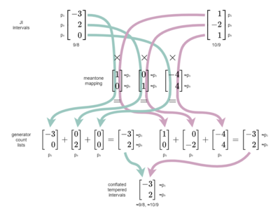
Sometimes it may be more helpful to imagine slicing your mapping matrix the other way, by columns (vectors) corresponding to the different primes, rather than rows (covectors) corresponding to generators.
And so we can see that tempering has reduced the dimensionality of our lattice by 1. Or in other words, the dimensionality of our lattice was always the rank; it’s just that in JI, the rank was equal to the dimensionality. And what’s happened by reducing this rank is that we eliminated one of the primes in a sense, by making it so we can only express things in terms of it via combinations of the other remaining primes.
rank and nullity
Let’s review what we’ve seen so far. 5-limit JI is 3-dimensional. When we have a rank-3 temperament of 5-limit JI, 0 commas are tempered out. When we have a rank-2 temperament of 5-limit JI, 1 comma is tempered out. When we have a rank-1 temperament of 5-limit JI, 2 commas are tempered out.[19]
There’s a straightforward formula here: [math]\displaystyle{ d - n = r }[/math], where [math]\displaystyle{ d }[/math] is dimensionality, [math]\displaystyle{ n }[/math] is nullity, and [math]\displaystyle{ r }[/math] is rank. We’ve seen every one of those words so far except nullity. Nullity simply means the count of commas tempered out, or in other words, the count of commas in a basis for the null-space (see Figure 5c).
So far, everything we’ve done has been in terms of 5-limit, which has dimensionality of 3. Before we generalize our knowledge upwards, into the 7-limit, let’s take a look at how things one step downwards, in the simpler direction, in the 3-limit, which is only 2-dimensional.
We don’t have a ton of options here! The PTS diagram for 3-limit JI could be a simple line. This axis would define the relative tuning of primes 2 and 3, which are the only harmonic building blocks available. Along this line we’ll find some points, which familiarly are ETs. For example, we find 12-ET. Its map here is ⟨12 19]; no need to mention the 5-term because we have no vectors that will use it here. At this ET, being a rank-1 temperament, [math]\displaystyle{ r }[/math] = 1. So if [math]\displaystyle{ d }[/math] = 2, then solve for [math]\displaystyle{ n }[/math] and we find that it only tempers out a single comma (unlike the rank-1 temperaments in 5-limit JI, which tempered out two commas). We can use our familiar null-space function to find what this comma is:
[math]\displaystyle{ \left[ \begin{array} {rrr} 12 & 19 \\ \hline 1 & 0 \\ 0 & 1 \end{array} \right] → \left[ \begin{array} {rrr} 12 & 228 \\ \hline 1 & 0 \\ 0 & 12 \end{array} \right] → \left[ \begin{array} {rrr} 12 & 0 \\ \hline 1 & -19 \\ 0 & 12 \end{array} \right] }[/math]
| input | output |
|---|---|
basis of NullSpace[{{12,19}}]
|
{-19,12} |
Unsurprisingly, the comma is [-19 12⟩, the compton comma. Basically, any comma we could temper out in 3-limit JI is going to be obvious from the ET’s map. Another option would be the blackwood comma, [-8 5⟩ tempered out in 5-ET, ⟨5 8]. Exciting stuff! Okay, not really. But good to ground yourself with.
But now you shouldn’t be afraid even of 11-limit or beyond. 11-limit is 5D. So if you temper 2 commas there, you’ll have a rank-3 temperament.
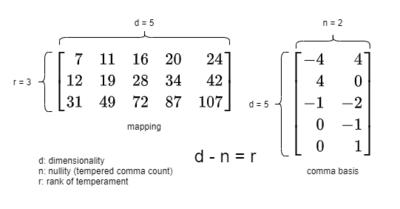
beyond the 5-limit
So far we’ve only been dealing with RTT in terms of prime limits, which is by far the most common and simplest way to use it. But nothing is stopping you from using other JI groups. What is a JI group? Well, I'll explain in terms of what we already know: prime limits. Prime limits are basically the simplest type of JI group. A prime limit is shorthand for the JI group consisting of all the primes up to that prime which is your limit; for example, the 7-limit is the same thing as the JI group "2.3.5.7". So JI groups are just sets of harmonics, and they are notated by separating the selected harmonics with dots.
Sometimes you may want to use a JI [[1]]. For example, you could create a 3D tuning space out of primes 2, 3, and 7 instead, skipping prime 5. You would call it “the 2.3.7 subgroup”. Or you could just call it "the 2.3.7 group", really. Nobody really cares that it's a subgroup of another group.
You could even choose a JI group with combinations of primes, such as the 2.5/3.7 group. Here, we still care about approximating primes 2, 3, 5, and 7, however there's something special about 3 and 5: we don't specifically care about approximating 3 or 5 individually, but only about approximating their combination. Note that this is different yet from the 2.15.7 group, where the combinations of 3 and 5 we care about approximating are when they're on the same side of the fraction bar.
As you can see from the 2.15.7 example, you don't even have to use primes. Simple and common examples of this situation are the 2.9.5 or the 2.3.25 groups, where you're targeting multiples of the same prime, rather than combinations of different primes.
And these are no longer JI groups, of course, but you can even use irrationals, like the 2.ɸ.5.7 group! The sky is the limit. Whatever you choose, though, this core structural rule [math]\displaystyle{ d - n = r }[/math] holds strong (see Figure 5d).
The order you list the pitches you're approximating with your temperament is not standardized; generally you increase them in size from left to right, though as you can see from the 2.9.5 and 2.15.7 examples above it can often be less surprising to list the numbers in prime limit order instead. Whatever order you choose, the important thing is that you stay consistent about it, because that's the only way any of your vectors and covectors are going to match up correctly!
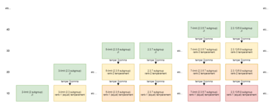
Alright, here’s where things start to get pretty fun. 7-limit JI is 4D. We can no longer refer to our 5-limit PTS diagram for help. Maps and vectors here will have four terms; the new fourth term being for prime 7. So the map for 12-ET here is ⟨12 19 28 34].
Because we're starting in 4D here, if we temper out one comma, we still have a rank-3 temperament, with 3 independent generators. Temper out two commas, and we have a rank-2 temperament, with 2 generators (remember, one of them is the period, which is usually the octave). And we’d need to temper out 3 commas here to pinpoint a single ET.
The particular case I’d like to focus our attention on here is the rank-2 case. This is the first situation we’ve been able to achieve which boasts both an infinitude of matrices made from comma vectors which can represent the temperament by its comma basis, as well as an infinitude of matrices made from ET maps which can represent a temperament by its mapping-row basis. These are not contradictory. Let’s look at an example: septimal meantone.
Septimal meantone may be thought of as the temperament which tempers out the meantone comma and the starling comma (126/125), or “meantone|starling”. But it may also be thought of as “meantone|marvel”, where the marvel comma is 225/224. We don’t even necessarily need the meantone comma at all: it can even be “starling|marvel”! This speaks to the fact that any temperament with a nullity greater than 1 has an infinitude of equivalent comma bases. It’s up to you which one to use.
On the other side of duality, septimal meantone’s mapping-row basis has two rows, corresponding to its two generators. We don’t have PTS for 7-limit JI handy, but because septimal meantone includes, or extends plain meantone, we can still refer to 5-limit PTS, and pick ETs from the meantone line there. The difference is that this time we need to include their 7-term. So the join of ⟨12 19 28 34] and ⟨19 30 44 53] would work. But so would ⟨19 30 44 53] and ⟨31 49 72 87]. We have an infinitude of options on this side of duality too, but here it’s not because our nullity is greater than 1, but because our rank is greater than 1.
canonical form
Recently we reduced
[math]\displaystyle{ \left[ \begin{array} {rrr} 5 & 8 & 12 \\ 7 & 11 & 16 \\ \end{array} \right] }[/math]
to
[math]\displaystyle{ \left[ \begin{array} {rrr} 1 & 1 & 0 \\ 0 & 1 & 4 \end{array} \right] }[/math]
The latter is sometimes called the “musician’s form” of the temperament, because it’s easy to reason about from a musical perspective. But it turns out there’s not a particularly clean function for consistently getting to it, or even defining it.
Another form you might want the mapping-row basis in is the type Graham Breed's temperament finder puts them in, where all values in a mapping-row basis row may be negative, but this is in the service of the generator being less than half the size of the period. For example, for meantone, we'd want the fourth instead of the fifth, and we can see that
[math]\displaystyle{ \left[ \begin{array} {rrr} 1 & 2 & 4 \\ 0 & -1 & -4 \end{array} \right] }[/math]
maps the fourth (4/3, [2 -1 0⟩) to [0 1⟩.
It’s often the case that a temperament’s nullity is greater than 1 or its rank is greater than 1, and therefore we have an infinitude of equivalent ways of expressing the comma basis or the mapping-row basis. This can be problematic, if we want to efficiently communicate about and catalog temperaments. It’s good to have a standardized form in these cases. The approach RTT takes here is to get these matrices into “canonical” form. In plain words, this just means: we have a function which takes in a matrix and spits out a matrix of the same shape, and no matter which matrix we input from a set of matrices which we consider all to be equivalent to each other, it will spit out the same result. This output is what we call the “canonical” matrix, and it can therefore uniquely identify a temperament.
To be clear, canonical form isn’t necessary to avoid ambiguity: you will never find a comma basis that could represent more than one temperament.
I've seen many specialized matrix forms used in RTT for problems like this, such as Smith normal form, Hermite Normal Form, Hermite Canonical Form, and maybe others. What we will be using here is "integer canonical form".[20].
For example, the canonical form of meantone is:
[math]\displaystyle{ \left[ \begin{array} {rrr} 1 & 0 & -4 \\ 0 & 1 & 4 \end{array} \right] }[/math]
If you take the integer canonical form of [⟨5 8 12] ⟨7 11 16]⟩, that’s what you get. It’s also what you get if you take the integer canonical form of [⟨12 19 28] ⟨19 30 44]⟩, etc. That’s the power of canonicalization.
To find the integer canonical form, we can combine the two processes we already know how to do: null-space for getting from a mapping-row basis to a comma basis, and anti-null-space to get from a comma basis to a mapping-row basis. Basically, to achieve canonical form of one type of basis, we convert it into the other type of basis, then back, and voilà: canonicalization.
For this, we need to up our game to Wolfram computable notebooks. You can click "Make Your Own Copy" in the top left of the screen if you want to modify this notebook to make your own calculations.
| input | output |
|---|---|
antiTranspose[m_] := Transpose[Reverse[m,{1,2}]]
|
{{1,0,-4},{0,1,4}}
{{-44,-30},{0,19},{19,0}} |
multimaps & multicommas
If you spend much time exploring information about RTT online, it won’t be long until you come across “wedgies”, which are an alternative way to represent temperaments. You may not need them to do RTT stuff; a lot of the information you can get from them can be gotten otherwise from the already-discussed matrices. But you may find they appeal to you. This section covers those.
multimaps
The mathematical structure used to represent a wedgie is called a multicovector, and this structure is indeed related to the mathematical structure called the “covector”:
- They both represent information written horizontally, as a row.
- They both use left angle brackets on the left and square brackets on the right, ⟨], to enclose their contents.
- They both exist on the left half of tuning duality, on the side built up out of ETs which concerns rank (not the side built up out of commas, which uses vectors/columns, and concerns nullity).
The main difference between the two is superficial, and has to do with the “multi” part of the name. A plain covector comes in only one type, but a multicovector can be a bicovector, tricovector, tetracovector, etc. Yes, a multicovector can even be a monocovector. Depending on its numeric prefix, a multicovector will be written with a different count of brackets on either side. For example, a bicovector uses two of each: ⟨⟨ ]]. A tricovector uses three of each: ⟨⟨⟨ ]]]. A monocovector, written with one of each, like ⟨], is indistinguishable from a plain covector, and that’s okay.
In order to make these materials as accessible as possible, I have been doing what I can to lean away from RTT jargon and instead toward generic, previously established mathematical and/or musical concepts. That is why I have avoided the terms "monzo", "val", "breed", and why I will now avoid "wedgie". When established mathematical and/or musical concepts are unavailable, we can at least use unmistakable analogs built upon what we do have. In this case, if in RTT we use covectors to represent maps, then analogously, we can refer to the thing multicovectors represent in RTT as a multimap.
So we mentioned that a multimap is an alternative way to represent a temperament. Let's look at an example now. Meantone's multimap looks like this: ⟨⟨ 1 4 4 ]]. As you can see, it is a bicovector, or bimap, because it has two of each bracket.
Why care about multimaps? Well, a key reason is that they can serve the same purpose as the canonical form of a temperament’s mapping-row basis: the process for converting a mapping-row basis to a multimap will convert any equivalent mapping-row basis to the same exact multimap. In other words, a multimap can serve as a unique identifier for its temperament.
Alright, then, sounds great! But how do I convert a mapping-row basis to a multimap? The process is doable. It’s closely related to the wedge product[21] (hence the name “wedgie”), which we write it with the symbol ∧.
First I’ll list the steps. Don’t worry if it doesn’t all make sense the first time. We’ll work through an example and go into more detail as we do. To be clear, what we're doing here is both more and less and different ways from the strict definition of the wedge product as you may see it elsewhere; I'm specifically here describing the process for finding the multimap in the form you're going to be interested in for RTT purposes.
- Take each combination of [math]\displaystyle{ r }[/math] primes where [math]\displaystyle{ r }[/math] is the rank, sorted in lexicographic order, e.g. if we're in the 7-limit, we'd have [math]\displaystyle{ (2,3,5) }[/math], [math]\displaystyle{ (2,3,7) }[/math], [math]\displaystyle{ (2,5,7) }[/math], and [math]\displaystyle{ (3,5,7) }[/math].
- Convert each of those combinations to a square [math]\displaystyle{ r×r }[/math] matrix by slicing a column for each prime out of the mapping-row basis and putting them together.
- Take each matrix's determinant.
- Set the results inside [math]\displaystyle{ r }[/math] brackets.
And you've got your multimap!
Another way to think about this is that you've found all of the minors of the matrix, where a minor is the determinant of a square submatrix. So we can think of multimaps as lists of minors.
Now, if you want the canonical multimap, two further steps are required:
- Change the sign of every result if the first non-zero result is negative.
- Extract the GCD from these results.
Let’s work through these steps for the example of meantone.
We have rank [math]\displaystyle{ r }[/math] = 2, so we’re looking for every combination of two primes. That’s out of the three total primes we have in the 5-limit: 2, 3, and 5. So those combinations are [math]\displaystyle{ (2,3) }[/math], [math]\displaystyle{ (2,5) }[/math], and [math]\displaystyle{ (3,5) }[/math]. Those are already in lexicographic order, or in other words, just like how alphabetic order works, but generalized to work for size of numbers too (so that 11 comes after 2, not before).
Here's the meantone mapping-row basis again, with some color applied which should help identify the combinations:
[math]\displaystyle{ \begin{bmatrix} \color{red}1 & \color{lime}0 & \color{blue}-4 \\ \color{red}0 & \color{lime}1 & \color{blue}4 \\ \end{bmatrix} }[/math]
So now each of those combinations becomes a square matrix, made out of bits from the mapping-row basis, which again is:
[math]\displaystyle{ \begin{array}{ccc} \text{(2,3)} & \text{(2,5)} & \text{(3,5)} \\ \begin{bmatrix}\color{red}1 & \color{lime}0 \\ \color{red}0 & \color{lime}1 \end{bmatrix} & \begin{bmatrix}\color{red}1 & \color{blue}-4 \\ \color{red}0 & \color{blue}4 \end{bmatrix} & \begin{bmatrix}\color{lime}0 & \color{blue}-4 \\ \color{lime}1 & \color{blue}4 \end{bmatrix} \end{array} }[/math]
Now we must take each matrix’s determinant. For 2×2 matrices, this is quite straightforward.
[math]\displaystyle{ \begin{bmatrix} a & b \\ c & d \end{bmatrix} → ad - bc }[/math]
So the three determinants are
[math]\displaystyle{ (1 × 1) - (0 × 0) = 1 - 0 = 1 \\ (1 × 4) - (-4 × 0) = 4 - 0 = 4 \\ (0 × 4) - (-4 × 1) = 0 + 4 = 4 }[/math]
So just set these inside a number brackets equal to the rank, and we’ve got ⟨⟨ 1 4 4 ]].
Wolfram Alpha won't be able to put the answer in brackets for you, but it can calculate the list of minors at least. The only trick is that you have to tell it the rank of your matrix as the second argument:
| input | output |
|---|---|
Minors[{{1,0,-4},{0,1,4}}, 2]
|
{{1, 4, 4}} |
Let's go for the canonical multimap. The first term is positive, so no sign changes are necessary. And these have no GCD, or in other words, their GCD is 1. So we're already there.
This method even works on an equal temperament, e.g. ⟨12 19 28]. The rank is 1 so each combination of primes has only a single prime: they’re [math]\displaystyle{ (2) }[/math], [math]\displaystyle{ (3) }[/math], and [math]\displaystyle{ (5) }[/math]. The square matrices are therefore [math]\displaystyle{ \begin{bmatrix}12\end{bmatrix} \begin{bmatrix}19\end{bmatrix} \begin{bmatrix}28\end{bmatrix} }[/math]. The determinant of a 1×1 matrix is defined as the value of its single term, so now we have 12 19 28. [math]\displaystyle{ r }[/math] = 1, so we set the answer inside one layer of brackets, so our monocovector is ⟨12 19 28].
| input | output |
|---|---|
Minors[{{12,19,28}}, 1]
|
{{12, 19, 28}} |
Going for the canonical multimap, we check that the leading term is positive, and no GCD. Both yes. So, this looks the same as what we started with, which is fine.
Let’s try a slightly harder example now: a rank-3 temperament, and in the 7-limit. There are four different ways to take 3 of 4 primes: [math]\displaystyle{ (2,3,5) }[/math], [math]\displaystyle{ (2,3,7) }[/math], [math]\displaystyle{ (2,5,7) }[/math], and [math]\displaystyle{ (3,5,7) }[/math].
If the mapping-row basis is
[math]\displaystyle{ \begin{bmatrix} \color{red}1 & \color{lime}0 & \color{blue}1 & \color{magenta}4 \\ \color{red}0 & \color{lime}1 & \color{blue}1 & \color{magenta}-1 \\ \color{red}0 & \color{lime}0 & \color{blue}-2 & \color{magenta}3 \\ \end{bmatrix} }[/math]
then the combinations are
[math]\displaystyle{ \begin{array}{ccc} \text{(2,3,5)} & \text{(2,3,7)} & \text{(2,5,7)} & \text{(3,5,7)} \\ \begin{bmatrix}\color{red}1 & \color{lime}0 & \color{blue}1 \\ \color{red}0 & \color{lime}1 & \color{blue}1 \\ \color{red}0 & \color{lime}0 & \color{blue}-2 \end{bmatrix} & \begin{bmatrix}\color{red}1 & \color{lime}0 & \color{magenta}4 \\ \color{red}0 & \color{lime}1 & \color{magenta}-1 \\ \color{red}0 & \color{lime}0 & \color{magenta}3 \end{bmatrix} & \begin{bmatrix}\color{red}1 & \color{blue}1 & \color{magenta}4 \\ \color{red}0 & \color{blue}1 & \color{magenta}-1 \\ \color{red}0 & \color{blue}-2 & \color{magenta}3 \end{bmatrix} & \begin{bmatrix}\color{lime}0 & \color{blue}1 & \color{magenta}4 \\ \color{lime}1 & \color{blue}1 & \color{magenta}-1 \\ \color{lime}0 & \color{blue}-2 & \color{magenta}3 \end{bmatrix} \\ \end{array} }[/math]
The determinant of a 3×3 matrix is trickier, but also doable:
[math]\displaystyle{ \begin{bmatrix} a & b & c \\ d & e & f \\ g & h & i \\ \end{bmatrix} → a(ei - fh) - b(di - fg) + c(dh -eg) }[/math]
In natural language, that’s each element of the first row times the determinant of the square matrix from the other two columns and the other two rows, summed but with an alternating pattern of negation beginning with positive. If you ever need to do determinants of matrices bigger than 3×3, see this webpage. Or, you can just use an online calculator.
And so our results are [math]\displaystyle{ -2 }[/math], [math]\displaystyle{ 3 }[/math], [math]\displaystyle{ 1 }[/math], [math]\displaystyle{ -11 }[/math]. Set these inside triply-nested brackets, because it’s a trimap for a rank-3 temperament, and we get ⟨⟨⟨ -2 3 1 -11 ]]].
| input | output |
|---|---|
Minors[{{1,0,1,4},{0,1,1,-1},{0,0,-2,3}}, 3]
|
{{-2, 3, 1, -11}} |
Now for canonical form. We need the first term to be positive; this doesn’t make a difference in how things behave, but is done because it canonicalizes things (we could have found the result where the first term came out positive by simply changing the order of the rows of our mapping-row basis, which doesn’t affect how it works as a mapping at all, or mean there's anything different about the temperament). And so we change the signs[22], and our list ends up as [math]\displaystyle{ 2 }[/math], [math]\displaystyle{ -3 }[/math], [math]\displaystyle{ -1 }[/math], [math]\displaystyle{ 11 }[/math]. There's no GCD to extract. So now we have ⟨⟨⟨ 2 -3 -1 11 ]]].
As for getting from a multimap back to the mapping-row basis, you can solve a system of equations for that. Though it’s not easy and there may not be a unique solution. And you probably will never find yourself with a multimap but without a corresponding mapping-row basis anyway.
multicommas
You may have noticed that the canonical multimap for meantone, ⟨⟨ 1 4 4 ]], looks really similar to the meantone comma, [-4 4 -1⟩. This is not a coincidence.
To understand why, we have to cover a few key points:
- Just as a vector is the dual of a covector, we also have a multivector which is the dual of a multicovector. Analogously, we call the thing the multivector represents a multicomma.
- We can calculate a multicomma from a comma basis much in the same way we can calculate a multimap from a mapping-row basis
- We can convert between multimaps and multicommas using an operation called “taking the dual”[23], which basically involves reversing the order of terms and changing the signs of some of them.
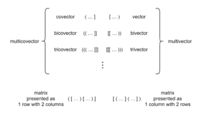
To demonstrate these points, let’s first calculate the multicomma from a comma basis, and then confirm it by calculating the same multicomma as the dual of its dual multimap.
Here’s the comma basis for meantone: ⟨[-4 4 -1⟩]. Calculating the multicomma is almost the same as calculating the multimap. The only difference is that as a preliminary step you must transpose[24] the matrix, or in other words, exchange rows and columns. In our bracket notation, that just looks like replacing ⟨[-4 4 -1⟩] with [⟨-4 4 -1]⟩. Now we can see that this is just like our ET map example from the previous section: basically an identity operation, breaking the thing up into three 1×1 matrices [math]\displaystyle{ \begin{bmatrix}-4\end{bmatrix} \begin{bmatrix}4\end{bmatrix} \begin{bmatrix}-1\end{bmatrix} }[/math] which are their own determinants and then nesting back inside one layer of brackets because nullity is 1. So we have [-4 4 -1⟩.
If we want the canonical multicomma, extracting any GCD is necessary. But unlike with the canonical multimap, we can't necessarily assume the leading term's sign will be positive. Since the canonical state is defined in terms of the canonical multimap, if we want to know the signs of the canonical multicomma, we'll have to find the canonical multimap. We can either separately find the canonical multimap, then take its dual, and that'd be our canonical multicomma. Or, we can take the dual of the multicomma we've found here, and if that has a negative leading term, then we just need to change the signs on both the multimap and the multicomma so they remain each other's duals but the multimap's leading term is positive, thus canonicalizing them together.
Now let’s see how to do the dual operation.
If your temperament's dimensionality [math]\displaystyle{ d }[/math] is 6 or less (within the 13-limit), you can take advantage of this table I've prepared, and use this simplified method:
- Find the correct cell in Figure 6b below using your temperament's [math]\displaystyle{ d }[/math] and [math]\displaystyle{ g }[/math], which stands for grade. Grade is like rank or nullity, but it is generic; if you are taking the dual of a multimap, you would use rank as the grade, and if you are taking the dual of a multicomma, you would use nullity as the grade. This cell should contain the same number of symbols as there are terms of your multimap.
- Match up the terms of your multimap with these symbols. If the symbol is [math]\displaystyle{ + }[/math], do nothing. If the symbol is [math]\displaystyle{ - }[/math], change the sign (positive to negative, or negative to positive; you could think of it like multiplying by either +1 or -1).
- Reverse the order of the terms.
- Set the result in the proper count of brackets.
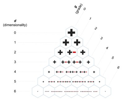
So in this case:
- We have [math]\displaystyle{ d=3 }[/math], [math]\displaystyle{ r=2 }[/math], so the correct cell contains the symbols [math]\displaystyle{ +-+ }[/math].
- Matching these symbols up with the terms of our multimap, we don't change the sign of 1, we do change the sign of 4 to -4, and we don't change the sign of the second 4.
- Now we reverse 1 -4 4 to 4 -4 1.
- Now we set the result in the proper count of brackets: [4 -4 1⟩
Ta-da! Both operations get us to the same result: [4 -4 1⟩.
What’s the proper count of brackets though? Well, the total count of brackets on the multicomma and multimap for a temperament must always sum to the dimensionality of the system from which you tempered. It’s the same thing as [math]\displaystyle{ d - n = r }[/math], just phrased as [math]\displaystyle{ r + n = d }[/math], and where [math]\displaystyle{ r }[/math] should be the bracket count for the multimap and [math]\displaystyle{ n }[/math] should be the bracket count for the multicomma. So with 5-limit meantone, with dimensionality 3, there should be 3 total pairs of brackets. If 2 are on the multimap, then only 1 are on the multicomma.
more on duals
Note the Pascal’s triangle shape to the numbers in Figure 6b. Also note that the mirrored results within each dimensionality are reverses of each other. Sometimes that means they’re identical, like [math]\displaystyle{ +-+-+ }[/math] and [math]\displaystyle{ +-+-+ }[/math]; other times not, like [math]\displaystyle{ +-++-+-+-+ }[/math] and [math]\displaystyle{ +-+-+-++-+ }[/math].
An important observation to make about multicommas and multimaps is that — for a given temperament — they always have the same count of terms. This may surprise you, since the rank and nullity for a temperament are often different, and the length of the multimap comes from the rank while the length of the multicomma comes from the nullity. But there’s a simple explanation for this. In either case, the length is not directly equal to the rank or nullity, but to the dimensionality choose the rank or nullity. And there’s a pattern to combinations that can be visualized in the symmetry of rows of Pascal’s triangle: [math]\displaystyle{ {d \choose n} }[/math] is always equal to [math]\displaystyle{ {d \choose {d - n}} }[/math], or in other words, [math]\displaystyle{ {d \choose n} }[/math] is always equal to [math]\displaystyle{ {d \choose r} }[/math]. Here are some examples:
| [math]\displaystyle{ d }[/math] | [math]\displaystyle{ r }[/math] | [math]\displaystyle{ d - r }[/math] | [math]\displaystyle{ {d \choose r} }[/math] | [math]\displaystyle{ {d \choose {d - r}} }[/math] | count |
|---|---|---|---|---|---|
| 3 | 2 | 1 | [math]\displaystyle{ (2,3) (2,5) (3,5) }[/math] | [math]\displaystyle{ (2) (3) (5) }[/math] | 3 |
| 4 | 3 | 1 | [math]\displaystyle{ (2,3,5) (2,3,7) (2,5,7) (3,5,7) }[/math] | [math]\displaystyle{ (2) (3) (5) (7) }[/math] | 4 |
| 5 | 3 | 2 | [math]\displaystyle{ (2,3,5) (2,3,7) (2,3,11) (2,5,7) (2,5,11) (2,7,11) (3,5,7) (3,5,11) (3,7,11) (5,7,11) }[/math] | [math]\displaystyle{ (2,3) (2,5) (2,7) (2,11) (3,5), (3,7) (3,11) (5,7) (5,11) (7,11) }[/math] | 10 |
Each set of one side corresponds to a set in the other side which has the exact opposite elements.
Note that multicommas could just as well serve the purpose of a unique identifier for temperaments. There’s no particular reason to prefer the canonical multimap to the canonical multicomma. By convention, however, the canonical multimap is the one that’s used.
If you need to do this process for a higher dimensionality than 6, then you'll need to understand how I found the symbols for each cell of Figure 6b. Here's how:
- Take the rank, halved, rounded up. In our case, [math]\displaystyle{ \lceil \frac{r}{2} \rceil = \lceil \frac{2}{2} \rceil = \lceil 1 \rceil = 1 }[/math]. Save that result for later. Let’s call it [math]\displaystyle{ x }[/math].
- Find the lexicographic combinations of [math]\displaystyle{ r }[/math] primes again: [math]\displaystyle{ (2,3) }[/math], [math]\displaystyle{ (2,5) }[/math], [math]\displaystyle{ (3,5) }[/math]. Except this time we don’t want the primes themselves, but their indices in the list of primes. So: [math]\displaystyle{ (1,2) }[/math], [math]\displaystyle{ (1,3) }[/math], [math]\displaystyle{ (2,3) }[/math].
- Take the sums of these sets of indices, and to each sum, also add [math]\displaystyle{ x }[/math]. So [math]\displaystyle{ 1+2+x }[/math], [math]\displaystyle{ 1+3+x }[/math], [math]\displaystyle{ 2+3+x }[/math] = [math]\displaystyle{ 1+2+1 }[/math], [math]\displaystyle{ 1+3+1 }[/math], [math]\displaystyle{ 2+3+1 }[/math] = [math]\displaystyle{ 4 }[/math], [math]\displaystyle{ 5 }[/math], [math]\displaystyle{ 6 }[/math].
- Even terms become [math]\displaystyle{ + }[/math]'s and odd terms become [math]\displaystyle{ - }[/math]'s.
Alternatively, you can just use this Wolfram Language computable notebook, which can calculate duals for you. It's a little trickier than other Wolfram Language tools shared here. I've basically recreated the multi(co)vector form in Wolfram with a tuple type where the first element is your multi(co)vector as a list of its terms, and the second element is its grade and variance. Variance[25] basically means which side of duality it is on. So variance is encoded via the sign of the grade, i.e. if this is a multivector, the grade is positive, and if it is a multicovector, then the grade is negative[26]. Again, grade is just generic rank or nullity, so it will simply be the count of brackets of your multi(co)vector.
| input | output |
|---|---|
eaIndices[d_,g_] := Subsets[Range[d],{g}]
|
{{31,49,72,87,107},-1}
{{107,-87,72,-49,31},4} |
tempered lattice fractions generated by prime combinations
So we now understand how to get to canonical multimaps. And we understand that they uniquely identify the temperament. But what about the individual terms — do they mean anything in and of themselves? It turns out: yes!
The first thing to understand is that each term of the canonical multimap pertains to a different combination of primes. We already know this: it’s how we calculated it from the mapping-row basis. For example, in the canonical multimap for meantone, ⟨⟨ 1 4 4 ]], the 1 is for [math]\displaystyle{ (2,3) }[/math], the first 4 is for [math]\displaystyle{ (2,5) }[/math], and the second 4 is for [math]\displaystyle{ (3,5) }[/math].
Now, let’s convert every term of the canonical multimap by taking its absolute value and its inverse. In this case, each of our terms is already positive, so that has no effect. But taking the inverse converts us to [math]\displaystyle{ \frac 11 }[/math], [math]\displaystyle{ \frac 14 }[/math], [math]\displaystyle{ \frac 14 }[/math]. These values tell us what fraction of the tempered lattice we can generate using the corresponding combination of primes.
What does that mean? Who cares? The motivation here is that it’s a good thing to be able to generate the entire lattice. We may be looking for JI intervals we could use as generators for our temperament, and if so, we need to know what primes to build them out of so that we can make full use of the temperament. So this tells us that if we try to build generators out of primes 2 and 3, we will succeed in generating [math]\displaystyle{ \frac 11 }[/math] or in other words all of the tempered lattice. Whereas if we try to build the generators out of primes 2 and 5, or 3 and 5, we will fail; we will only be able to generate [math]\displaystyle{ \frac 14 }[/math] of the lattice. In other words, prime 5 is the bad seed here; it messes things up.
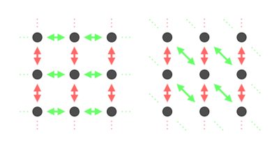
It’s easy to see why this is the case if you know how to visualize it on the tempered lattice. Let’s start with the happy case: primes 2 and 3. Prime 2 lets us move one step up (or down). Prime 3 lets us move one step right (or left). Clearly, with these two primes, we’d be able to reach any node in the lattice. We could do it with generators 2/1 and 3/1, in the most straightforward case. But we can also do it with 2/1 and 3/2: that just means one generator moves us down and to the right (or the opposite), and the other moves us straight up by one (or the opposite) (see Figure 6b). 2/1 and 4/3 works too: one moves us to the left and up two (or… you get the idea) and the other moves us straight up by one. Heck, even 3/2 and 4/3 work; try it yourself.
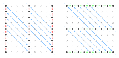
But now try it with only 5 and one other of primes 2 or 3. Prime 5 takes you over 4 in both directions. But if you have only prime 2 otherwise, then you can only move up or down from there, so you’ll only cover every fourth vertical line through the tempered lattice. Or if you only had prime 3 otherwise, then you could only move left and right from there, you’d only cover every fourth horizontal line (see Figure 6c).
One day you might come across a canonical multimap which has a term equal to zero. If you tried to interpret this term using the information here so far, you'd think it must generate [math]\displaystyle{ \frac 10 }[/math]th of the tempered lattice. That's not easy to visualize or reason about. Does that mean it generates essentially infinity lattices? No, not really. More like the opposite. The question itself is somewhat undefined here. If anything, it's more like that combination of primes generates approximately none of the lattice. Because in this situation, the combination of primes whose canonical multimap term is zero generates so little of the tempered lattice that it's completely missing one entire dimension of it, so it's an infinitesimal amount of it that it generates. For example, the 11-limit temperament 7&12&31 has canonical multimap ⟨0 1 1 4 4 -8 4 4 -12 -16] and mapping-row basis [⟨1 0 -4 0 -12] ⟨0 1 4 0 8] ⟨0 0 0 1 1]⟩; we can see from this how primes [math]\displaystyle{ (2,3,5) }[/math] can only generate a rank-2 cross-section of the full rank-3 lattice, because while 2 and 3 do the trick of generating that rank-2 part (exactly as they do in 5-limit meantone), prime 5 doesn't bring anything to the table here so that's all we get.
We’ll look in more detail later at how exactly to best find these generators, once you know which primes to make them out of.
other topics (TBD)
summary diagrams and tables
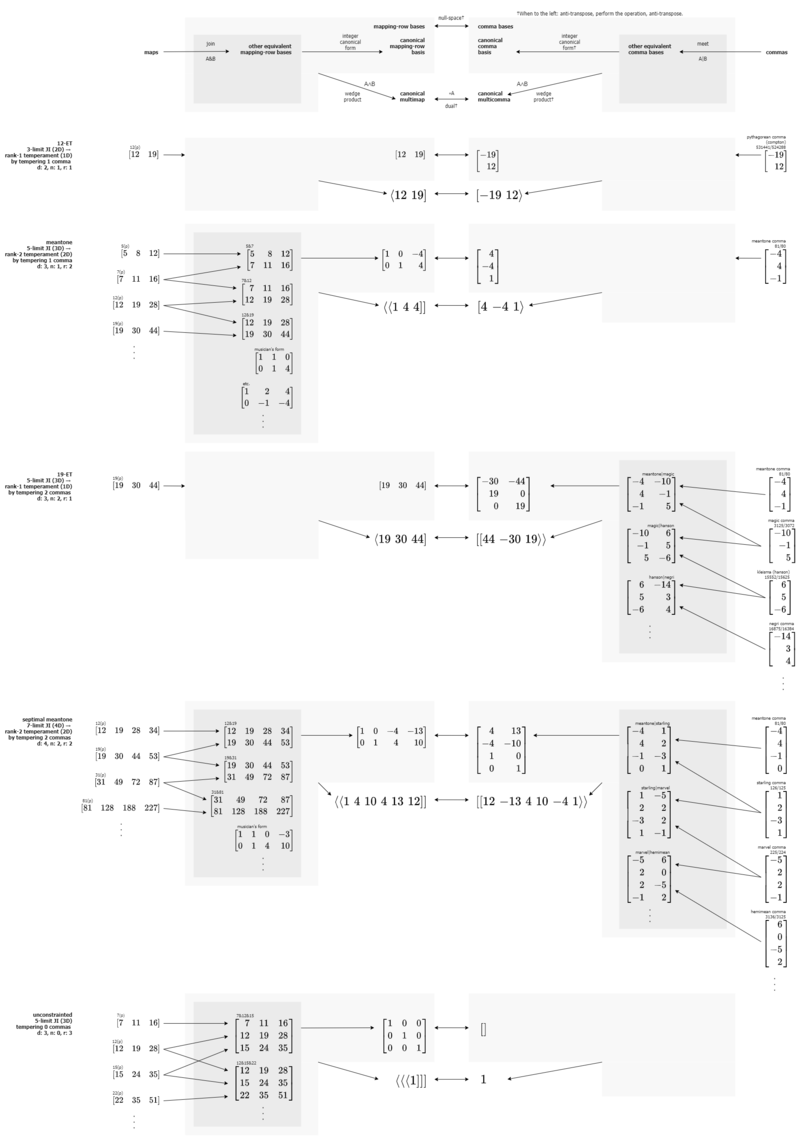
| terminology category | building block → | ways to identify a temperament | ← building block | |||
|---|---|---|---|---|---|---|
| RTT application | map, mapping-row (often an ET) | mapping, mapping-row basis | multimap | multicomma | comma basis | interval, comma |
| RTT structure | map | list of maps | list of minors | list of minors | list of prime count lists | prime count list |
| linear algebra structure | row vector, matrix row | matrix | minors row vector | minors (column) vector | matrix | (column) vector, matrix column |
| multilinear algebra structure[27] | covector | list of covectors | multicovector | multivector | list of vectors | vector |
| extended bra-ket notation representation | bra | ket of bras | nested bras | nested kets | bra of kets | ket |
| RTT jargon | val[28] | list of vals | wedgie, multival | multimonzo | list of monzos | monzo |
tuning
scales
lattices
finding approximate JI generators
non-octave periods
outro
You’ve made it to the end. This is pretty much everything that I understand about RTT at this point (May 2021). This took me a little over a month of full-time funemployed exploration to learn and put together; at the onset, while having considered myself a xenharmonicist for 15 years, I only understood a few scattered things about RTT, such as ET maps and commas and the overlapping MOS concepts. I hope that equipped with my results here it shouldn’t take a newcomer nearly that much time to get going. And of course I hope to continue learning more myself and perhaps even contributing to the theory one day, since there’s still plenty of frontier here.
I couldn’t have put this together without the help of:
- Paul Erlich
- Mike Battaglia
- Graham Breed
- Dave Keenan
- Steve Martin
- Herman Miller
- Keenan Pepper
- Scott Thompson
- Joshua Sanchez
- Vincenzo Sicurella
- Petr Pařízek
- Margo Schulter
- Stephen Weigel
plus many many more. And of course I owe a big debt to Gene Ward Smith.
I take full responsibility for any errors or shortcomings of this work. Please feel free to edit this stuff yourself if you have something you'd like to correct, revise, or contribute.
Happy tempering!
- ↑ And curiously little about the history.
- ↑ This list of logarithmic identities has been an excellent resource for me in getting my head around logarithmic thinking. As you can see there, [math]\displaystyle{ \frac{log_{10}{a}}{log_{10}{b}} = log_{b}{a} }[/math], so the base doesn't matter; you could put anything in there — 10, 2, e — and it still reduces to [math]\displaystyle{ log_{b}{a} }[/math].
- ↑ For more information, see: The Riemann zeta function and tuning.
- ↑ My main concern with the term "generalized patent val", or GPV, is that it gets things backwards: it posits the GPV as a type of patent val, when it makes more sense to think of it the other way around, with the patent val as a type of GPV.
The present definition of GPV on the wiki bends over backwards to make its way work, essentially using non-integer EDOs, which are a contradiction in terms. Consider this alternative definition, however, which is more straightforward:
A GPV is any relatively near-just map found by uniformly multiplying the generators for JI (⟨log₂2 log₂3 log₂5 ... ]) by any value before rounding it to integers. For example, choosing 17.1, we find the map 17.1⟨1 1.585 2.322] = ⟨17.1 27.103 39.705] which rounds to ⟨17 27 40]. This is one of the many GPVs for 17-EDO, and every EDO has many possible GPVs. To find a GPV for n-EDO, choose any multiplier that rounds to n; another example for 17-EDO could be 16.9⟨1 1.585 2.322] = ⟨16.9 26.786 39.241] which rounds to ⟨17 27 39].
The key element in this definition is the uniform multiplier, and from it we draw our proposed replacement name for this structure: a uniform map. So the definition could be:
A uniform map is any relatively near-just map found by uniformly multiplying the generators for JI (⟨log₂2 log₂3 log₂5 ... ]) by any value before rounding it to integers. For example, choosing 17.1, we find the map 17.1⟨1 1.585 2.322] = ⟨17.1 27.103 39.705] which rounds to ⟨17 27 40]. This is one of the many uniform maps for 17-EDO, and every EDO has many possible uniform maps. To find a uniform map for n-EDO, choose any multiplier that rounds to n; another example for 17-EDO could be 16.9⟨1 1.585 2.322] = ⟨16.9 26.786 39.241] which rounds to ⟨17 27 39].
Any uniform map whose multiplier is an integer — or "integer uniform map" — is always the simple map for the corresponding EDO. And every simple map is also an integer uniform map. These are just two different helpful ways of thinking about the same structure; in contexts pertaining to tuning accuracy, "simple map" works great, and in contexts pertaining to other uniform maps, "integer uniform map" works great. - ↑ My first concern with “patent” map is that "patent", as an adjective, is unfamiliar to most people, unless it relates to those documents called patents. Calling them "obvious maps" would have been better than "patent maps".
The second concern is that they are not always obvious. If it were, there would be no contention about it. This name suggests a positive value judgment (and dismissive value judgement on other maps) which we think is inappropriate. A name like “patent” or "obvious" map may lead too many people concerned with accurate tuning to accept this map when if they'd known better they may have preferred the map with the most accurate tuning overall, i.e. the “best” map. The classic example of a best map which is not the patent map is 17c at the 5-limit.
These concerns arose in recent public discussion I was involved in, and it was agreed at that time that "naive" was an apt replacement for "patent". But through further discussion, we decided that this would have the opposite problem: where "patent" had excessively positive connotations, "naive" would have had inappropriately negative connotations, and might run the risk of discouraging people from using them despite such maps being relatively good. So we concluded that a word with more neutral connotations was appropriate, and so we're going with "simple". These maps may not always be obvious, but they are always simple to calculate.
The simple map sets octaves pure, and then for each other prime harmonic individually, chooses the nearest mapping (the one with least error). That's clearly simple, and it's good, but it's not necessarily best. On the other hand, the best map is not strictly defined yet, but it would have a more elaborate definition, involving a consideration of errors in the ratios between primes, not only in the primes themselves. - ↑ On some versions of PTS which Paul prepared, these contorted ETs are actually printed on the page.
- ↑ The reason is that Paul’s diagram, in addition to cutting off beyond 99-ET, also filters out maps that aren’t GPVs.
- ↑ Yes, these are the same as the Pythagorean comma and Pythagorean diatonic semitone, respectively.
- ↑ There’s an extension of this pattern. Pick any ET. Maybe start with a prominent one like 7, or 12. Notice that you can find lines radiating out from it of aligned ETs. These would all be rank-2 temperaments, though they’re not all drawn. You’ll see that if you pick any size of numeral and follow consecutive numerals of continuously changing size, that the values decrease by the ET number you’re radiating out from. That’s because each step you can think of subtracting that ET number over and over, because moving inward you’d be doing the opposite: repeatedly adding that ET number, per the rules of the scale tree.
- ↑ Each tier of the Stern-Brocot tree is the next Farey sequence.
- ↑ This statement is slightly misleading, in order to help make the more important point it's in the context of. The full truth is that augmented's period is 400¢ at 12-ET. As you'll soon seen, the period is just a special name for the first one of a temperament's generators, but because in rank-2 situations like this where there are only two generators, referring to the generator typically implies the second generator, the one which is not the period. For augmented, this generator is 100¢ at 12-ET.
- ↑ As you can confirm using the matrix tools you'll learn soon, technically speaking you can temper them both out at the same time... but it'll only be by using 0-EDO, i.e. a system with only a single pitch. For more information see trivial temperaments.
- ↑ Elsewhere, you may see this described as "cross-breeding", where an ET map is a "breed".
- ↑ To be clear, because what you are adding and subtracting in interval vectors are exponents (as you know), the commas are actually being multiplied by each other; e.g. [-4 4 -1⟩ + [10 1 -5⟩ = [6 5 -6⟩, which is the same thing as [math]\displaystyle{ \frac{81}{80} × \frac{3072}{3125} = \frac{15552}{15625} }[/math]
- ↑ Bra-ket notation comes to RTT from quantum mechanics, not algebra.
- ↑ Besides, in most contexts the null-space of a linear mapping is thought of as a list of vectors, rather than a matrix, but it’s generally more helpful for us here to think of it smooshed together as a matrix.
- ↑ i.e. we might have expected it to return {{-44,-30},{0,19},{19,0}} instead of {{-44,0,19},{-30,19,0}}. That's why if you look carefully at the Wolfram Language example given earlier, we define our custom nullSpaceBasis function to include a Transpose (it also includes a Reverse, which swaps the order of the commas, to get the lowest prime-limit ones first).
- ↑ For real numbers [math]\displaystyle{ p,q }[/math] we can make the two generators respectively [math]\displaystyle{ \frac{p}{5p+7q} }[/math] and [math]\displaystyle{ \frac{q}{5p+7q} }[/math] of an octave, e.g. [math]\displaystyle{ (p,q)=(1,0) }[/math] for 5-ET, [math]\displaystyle{ (0,1) }[/math] for 7-ET, [math]\displaystyle{ (1,1) }[/math] for 12-ET, and many other possibilities.
- ↑ Probably, a rank-0 temperament of 5-limit JI would temper 3 commas out. All I can think a rank-0 temperament could be is a single pitch, or in other words, everything is tempered out. So perhaps in some theoretical sense, a comma basis in 5-limit made out of 3 vectors, thus a square 3×3 matrix, as long as none of the lines are parallel, should minimally represent every interval in the space.
- ↑ Historically, Hermite Normal Form was used as if it gave a unique identifier for each temperament, when in fact it did not. It failed to remove possibly-hidden common factors in the columns of comma bases and rows of mapping-row bases, leading to situations which were named "torsion" and "contorsion", respectively. Hermite Canonical Form goes too far it reduces the matrix's diagonals to all 1's or 0's, which loses important information for temperaments with non-octave periods. Integer canonical form removes such common factors without compromising non-octave periods, therefore truly giving a unique identifier, and also eliminating the need to deal with torsion or contorsion.
- ↑ The wedge product is also known as the exterior product. Exterior and interior products (∧ and ⨼) should not be confused with outer and inner products, which in RTT are ordinary matrix products between a vector and a covector. The outer product gives a matrix and the inner product a scalar. e.g. [1 2⟩⟨3 4] = ⟨[3 4⟩ [6 8⟩] and ⟨3 4][1 2⟩ = 11. In our application, the inner product is the same as the dot product used for maps and intervals.
- ↑ If it helps you, you could think of this sign-changing step as paired with the GCD extraction step, if you think of it like extracting a GCD of -1.
- ↑ This operation uses the same process as is used for finding the complement in exterior algebra, however, whereas exterior algebra does not convert between vectors and covectors (it can be used on either one, staying within that category), with RTT's dual you switch which type it is as the last step. More details can be found below. The dual we use in RTT is #2 in the table. It essentially combines elements from both #1 and #3.
Table 6(footnote). Three similar duals # dual type notes variance changing using RTT's extended bra-ket notation to operator example alternate example example (ASCII only) alternate example (ASCII only) 1 Grassman/EA/orthogonal complement also called "dual" within EA, but "complement" is preferred to avoid confusion with the variance-changing MLA dual no demonstrate agnosticism to and unchanging of variance negation, overbar, tilde ¬[1 4 4⟩ = [4 -4 1⟩ [̅1̅ ̅4̅ ̅4̅⟩ = [4 -4 1⟩ ~[1 4 4> = [4 -4 1> 2 MLA dual, in EA form compresses the antisymmetric/skew-symmetric matrix/tensor into a list of minors; this is the dual that RTT uses yes distinguish covariance from contravariance asterisk ∗⟨⟨1 4 4]] = [4 -4 1⟩ *<<1 4 4]] = [4 -4 1> 3 MLA dual, in tensor form uses the full antisymmetric/skew-symmetric matrix/tensor itself; here this operation is known as the Hodge dual yes distinguish covariance from contravariance Hodge star ⋆⟨⟨0 1 4] ⟨-1 0 4] ⟨-4 -1 0]] = [4 -4 1⟩ ⋆[[0 1 4] [-1 0 4] [-4 -1 0]]⁰₂ = [4 -4 1]¹₀ *<<0 1 4] <-1 0 4] <-4 -1 0]] = [4 -4 1> *[[0 1 4] [-1 0 4] [-4 -1 0]] type (1,1) = [4 -4 1] type (1,0)) - ↑ Or do an anti-transpose sandwich, if you want to be consistent with other operations discussed here; either way will work here.
- ↑ (Multi)covectors are covariant, while (multi)vectors are contravariant. This has to do with how vectors vary with respect to the system's units. Covectors vary in the same direction as the units, hence the co- prefix meaning "with", while (contra)vectors vary in the opposite direction to the units, hence the contra- prefix meaning "against".
- ↑ If the grade is zero, you probably don't need this tool, but it is capable of handling this case! When the grade is zero, it has no way to figure the dimensionality of the system (in other cases it calculates it based on the lenght of the multi(co)vector), so you must provide that yourself. So as a second argument, simply provide the grade and variance of the target dual. For example, if you have the multivector for JI (where nothing is tempered out), {{1}, 0}, there's no way to tell what prime limit you're in; so if you're in 5-limit, you would use dual[{{1}, 0}, -3], because you know the grade of the dual multicovector is 3 and it should be negative because multicovectors encode their variance as a negative sign on the grade here. One last point here: multi(co)vectors with grade 0 are neither covariant nor contravariant, in other words they are neither covectors nor vectors; they are simply scalars, and so you can actually call this like dual[{1, 0}, -3] if you prefer.
- ↑ RTT uses multilinear algebra structures, but does not use the conventional tensor (multi-dimensional array) representations of them; instead, it uses two copies of exterior algebra, one on each side of the duality, and an extended version of bra-ket notation. In other words, you can think of the multi(co)vectors used in RTT as compressed forms of antisymmetric tensors. A tensor is like a multi-dimensional array, or you could think of it as a generalization of matrices to other dimensions besides 2. And confusingly, antisymmetric doesn't mean the non-symmetric or undoing symmetry; it is a specific type of symmetry. This is made clearer in another name for antisymmetric, which is skew-symmetric. This reveals that the type of symmetry these tensors exhibit is along a skew, or diagonal. Let's take the example of meantone. Technically speaking, when you take the wedge product of two vectors (or covectors), the result is a matrix: [math]\displaystyle{ \left[ \begin{array} {rrr} 0 & 1 & 4 \\ -1 & 0 & 4 \\ -4 & -4 & 0 \\ \end{array} \right] }[/math] But this isn't a particularly efficient representation of this information. Everything in the bottom left triangular half is a mirror of what's in the top right triangular half, just with the signs changed! We compress this as ⟨⟨ 1 4 4 ]] instead, leveraging the antisymmetry. For a higher dimensional temperament, the tensor representation would be a higher-dimensional square, such as a cube, hypercube, 5-cube, etc. and the antisymmetry would lead to one tetrahedral, 4-simplex, 5-simplex, etc. half being mirrored but with signs changed. So we compress it into a multicovector with even more brackets. No big deal.
- ↑ "Val" creates an unnecessary barrier to understanding for those already familiar with established terms for concepts RTT borrows from linear algebra. Even if it does have some connection to the mathematical concept of a "valuation", this is of no help in illuminating its music-theory meaning, which is simply that of being a mapping from a single generator to primes. The first sentence in the Xenharmonic Wiki article for "val" says, "a val is a linear map". And the first sentence of the Wikipedia article where "covector" redirects to is: "... a covector is a linear map from a vector space to its field of scalars". So that is why we use "map" in this material instead.