Dave Keenan & Douglas Blumeyer's guide to EA for RTT
This article is meant as an introduction to exterior algebra (EA)[note 1] as it was developed for use in regular temperament theory primarily by Gene Ward Smith, and works as a supplement to Dave Keenan & Douglas Blumeyer's guide to RTT. It also includes some concepts from multilinear algebra.
A very brief history
In the very earliest days of the modern paradigm, regular temperaments were expressed in matrix form[note 2], and most needs—mapping, tuning, complexity measurement, etc.—were fielded by basic linear algebra tools. Soon thereafter Gene Ward Smith began contributing several more mathematically advanced innovations to the developing theory, in particular the use of EA tools such as the wedge product[note 3]. In the present day, a mix of linear algebra and exterior algebra tools are used in the RTT community; most things that can be done by one of the two algebras can be done to at least some extent by the other, and preferences differ from one theoretician to the other as to which style to use.
Introduction
From vectors to multivectors
If you have browsed around the regular temperaments part of this wiki before, it's likely that you've come across the wedgie, which is a special way to represent a regular temperament.
The mathematical structure used to represent a wedgie is called a multicovector, and this structure is indeed related to the mathematical structure called the covector (also called a linear form). Like how a (co)vector is an element in linear algebra, a multi(co)vector is an element in exterior algebra. You are likely familiar with covectors already due to their use for representing maps in RTT, such as the map for 5-limit 12-ET, ⟨12 19 28]. A good introductory example of a multicovector would be the wedgie for meantone: ⟨⟨ 1 4 4 ]].
Covectors and multicovectors both:
- Represent information written horizontally, as a row.
- Use left angle brackets on the left and square brackets on the right, ⟨…], to enclose their contents.
- Exist on the left half of tuning duality, on the side built up out of ETs which concerns rank (not the side built up out of commas, which uses vectors/columns, and concerns nullity).
- Have a dual structure with the same name minus the "co" part.
The main difference between the two is somewhat superficial, and has to do with the “multi” part of the name. A plain covector comes in only one type, but a multicovector can be a bicovector, tricovector, quadricovector, etc. Yes, a multicovector can even be a plain covector, which can be called a monocovector when there might otherwise be ambiguity. A multicovector can even be a nilocovector[note 4] (a scalar).
Depending on its numeric prefix, a multicovector will be written with a different count of brackets on either side[note 5]. For example, a bicovector uses two of each: ⟨⟨ … ]]. A tricovector uses three of each: ⟨⟨⟨ … ]]]. And of course a (mono)covector is written with one of each, like ⟨…]. And a nilocovector, with zero brackets, is indistinguishable from a simple scalar. As you can see, our meantone example is a bicovector, because it has two of each bracket.
Just as covectors have dual structures called vectors, multicovectors have duals which are called multivectors. When we need to refer to multivectors and multicovectors in the general case, we call them "varianced multivectors"[note 6]. Which brings us to our next section: on variance.
Variance
Multivectors and multicovectors cannot be arbitrarily mixed; it is of critical importance to keep track of which type one is. To convert between a multivector and its dual multicovector, we use a "dual" function. This function is discussed later in this article.
Variance is a word which captures this notion of duality, because multicovectors are covariant, while multivectors are contravariant.[note 7] For more information, see variance.
As compressed antisymmetric tensors
You can think of the varianced multivectors used in RTT as compressed forms of antisymmetric tensors, a concept that comes to us from MLA[note 8]. Let's define both of those words.
A tensor is like a multi-dimensional array, or you could think of it as a generalization of square matrices to other dimensions besides 2, i.e. cubes, hypercubes, etc.
And as for antisymmetric, we should first say that a symmetric tensor is one that remains unchanged if you swap any two of its dimensions[note 9], for example transposing a 2D matrix so that its rows become columns and vice versa. So an antisymmetric tensor is one that becomes its own negation, i.e. the signs of all the numbers change, if you swap any two of its dimensions.

To visualize how, let's take that example of meantone again. For these purposes, ignore variance; we'll just use the terms multivector and vector here. So, while in RTT materials the wedge product (from where "wedgie" gets its name) is described as returning a multivector, in EA (which is where the wedge product comes to us from), when you take the wedge product of two vectors, the result looks like a matrix but is really a bivector represented in tensor form, as a tensor of order 2:
[math]\displaystyle{ \left[ \begin{array} {rrr} 0 & 1 & 4 \\ -1 & 0 & 4 \\ -4 & -4 & 0 \\ \end{array} \right] }[/math]
But as you can see, this isn't a particularly efficient representation of this information. It exhibits a lot of redundancy. Everything in the bottom left triangular half is a mirror of what's in the top right triangular half, just with the signs changed. This is the aforementioned antisymmetry! So, in RTT, we compress this as the multivector ⟨⟨ 1 4 4 ]] instead, leveraging the antisymmetry.
For a higher dimensional temperament, the tensor representation would be a higher-dimensional square, such as a cube, hypercube, 5-cube, etc. and the antisymmetry would lead to one tetrahedral, 4-simplex, 5-simplex, etc. half being mirrored but with signs changed. So we compress it into a multivector with even more brackets. But no matter how many brackets, the multivectors in RTT will always be 1D strings of numerals, sorted in lexicographic order by their indices in the higher-dimensional square.
For more information, see: Wikipedia:Exterior algebra#Alternating tensor algebra.
Multimaps & multicommas
In everyday RTT, we don't usually need to use the words for the mathematical structures such as "covector" or "vector" which underpin our work. We usually simply refer to the musical objects that these mathematical objects represent, such as "maps", or "commas". Similarly, in EA, we can generally stick to using words closer to the domain application, so henceforth we will stick primarily with multimap[note 10], the object typically represented by a multicovector, and multicomma, the object typically represented by a multivector. This is an extrapolation from the terms "map" and "comma", which could be written as "monomap" and "monocomma" if necessary to distinguish them from other multimaps and multicommas, but generally can be shortened to "map" and "comma". A wedgie is a multimap. For example, a wedgie for a rank-2 temperament would be a bimap or 2-map.
When speaking of multimaps and multicommas in general, we still need the mathematical term "varianced multivector". But this is no different than how we use the term "varianced matrix" when speaking of mappings and comma bases in general.
In order to make these materials as accessible as possible, we will be doing what is possible to lean away from jargon and instead toward generic, previously established mathematical and/or musical concepts, especially descriptive ones. That is why we avoid the terms "monzo", "val", "breed", and "wedgie". When established mathematical and/or musical concepts are unavailable, we can at least use unmistakable analogs built upon what we do have.
Wolfram Language implementation
Dave and Douglas have also collaborated on producing a code library for RTT implemented in Wolfram Language, including functions for all major operations in EA form as well: eaDual[], eaCanonicalForm[], matrixToMultivector[], and multivectorToMatrix[], as well as helpers like eaDimensionality[], eaRank[], and eaNullity[].
The library represents varianced multivectors with a custom data structure. The first entry is its list of numerals. The second entry is its variance. The third entry is its grade, which is the generic word for rank or nullity, so you can think of it as the count of the angle brackets.[note 11].
The code is maintained and shared on GitHub here: https://github.com/cmloegcmluin/RTT
More details can be found on the README there.
Converting matrices to varianced multivectors
Basic steps for converting mapping to multimap
To begin, we’ll just list the steps. These steps work for converting a mapping to a multimap; if you're interested in converting a comma basis to a multicomma, that process is a variation on this process, and will be discussed at the end of this section. Don’t worry if it doesn’t all make sense the first time. We’ll work through several examples and go into more detail soon.
- Take each combination of r primes where r is the rank, sorted in lexicographic order, e.g. if we're in the 7-limit, we'd have (2, 3, 5), (2, 3, 7), (2, 5, 7), and (3, 5, 7).
- Convert each of those combinations to a square r×r matrix by slicing a column for each prime out of the mapping-row-basis and putting them together.
- Take each matrix's determinant.
- Set the results inside r brackets.
And you've got your multimap.
As alluded to earlier, the conversion process from a mapping to a multimap is closely related to the wedge product. But to be clear, what we're doing here is different from the strict definition of the wedge product as you may see it elsewhere. That is because we are going straight from a matrix representation, bypassing a tensor representation, and going straight for the varianced multivector representation.
More on the wedge product here: Varianced Exterior Algebra#The wedge product
Canonical form
Now, if you want the canonical multimap, two further steps are required:
- Change the sign of every result if the first non-zero result is negative.
- Divide each of these results by their GCD.
If your mapping is in canonical form as a matrix, the resultant multimap will already be the canonical multimap.
Examples
Rank-2
Let’s work through the steps broken out above, on our the example of meantone.
We have rank r = 2, so we’re looking for every combination of two primes. That’s out of the three total primes we have in the 5-limit: 2, 3, and 5. So those combinations are (2, 3), (2, ,5), and (3, 5). Those are already in lexicographic order, or in other words, just like how alphabetic order works, but generalized to work for size of numbers too (so that 11 comes after 2, not before).
Here's the meantone mapping-row-basis again, with some color applied which should help identify the combinations:
[math]\displaystyle{ \begin{bmatrix} \color{red}1 & \color{lime}0 & \color{blue}-4 \\ \color{red}0 & \color{lime}1 & \color{blue}4 \\ \end{bmatrix} }[/math]
So now each of those combinations becomes a square matrix, made out of bits from the mapping-row-basis, which again is:
[math]\displaystyle{ \begin{array}{ccc} \text{(2,3)} & \text{(2,5)} & \text{(3,5)} \\ \begin{bmatrix}\color{red}1 & \color{lime}0 \\ \color{red}0 & \color{lime}1 \end{bmatrix} & \begin{bmatrix}\color{red}1 & \color{blue}-4 \\ \color{red}0 & \color{blue}4 \end{bmatrix} & \begin{bmatrix}\color{lime}0 & \color{blue}-4 \\ \color{lime}1 & \color{blue}4 \end{bmatrix} \end{array} }[/math]
Now we must take each matrix’s determinant. For 2×2 matrices, this is quite straightforward.
[math]\displaystyle{ \begin{bmatrix} a & b \\ c & d \end{bmatrix} → ad - bc }[/math]
So the three determinants are
[math]\displaystyle{ (1 × 1) - (0 × 0) = 1 - 0 = 1 }[/math]
[math]\displaystyle{ (1 × 4) - (-4 × 0) = 4 - 0 = 4 }[/math]
[math]\displaystyle{ (0 × 4) - (-4 × 1) = 0 + 4 = 4 }[/math]
So just set these inside a number brackets equal to the rank, and we’ve got ⟨⟨ 1 4 4 ]].
Let's go for the canonical multimap. The first term is positive, so no sign changes are necessary. And these have no GCD, or in other words, their GCD is 1. So we're already there. Which is to be expected because we used the canonical form of the meantone mapping as input.
Rank-1 (equal)
This method even works on an equal temperament, e.g. ⟨12 19 28]. The rank is 1 so each combination of primes has only a single prime: they’re (2), (3), and (5). The square matrices are therefore [12] [19] [28]. The determinant of a 1×1 matrix is defined as the value of its single term, so now we have 12 19 28. Since r = 1, we set the answer inside one layer of brackets, so our monocovector is ⟨12 19 28].
Going for the canonical multimap, we check that the leading term is positive, and no GCD. Both yes. So, this looks the same as what we started with, which is fine.
Rank-3
Let’s try a slightly harder example now: a rank-3 temperament, and in the 7-limit. There are four different ways to take 3 of 4 primes: (2, 3, 5), (2, 3, 7), (2, 5, 7), and (3, 5, 7).
If the mapping-row-basis is
[math]\displaystyle{ \begin{bmatrix} \color{red}1 & \color{lime}0 & \color{blue}1 & \color{magenta}4 \\ \color{red}0 & \color{lime}1 & \color{blue}1 & \color{magenta}-1 \\ \color{red}0 & \color{lime}0 & \color{blue}-2 & \color{magenta}3 \\ \end{bmatrix} }[/math]
then the combinations are
[math]\displaystyle{ \begin{array}{ccc} \text{(2,3,5)} & \text{(2,3,7)} & \text{(2,5,7)} & \text{(3,5,7)} \\ \begin{bmatrix}\color{red}1 & \color{lime}0 & \color{blue}1 \\ \color{red}0 & \color{lime}1 & \color{blue}1 \\ \color{red}0 & \color{lime}0 & \color{blue}-2 \end{bmatrix} & \begin{bmatrix}\color{red}1 & \color{lime}0 & \color{magenta}4 \\ \color{red}0 & \color{lime}1 & \color{magenta}-1 \\ \color{red}0 & \color{lime}0 & \color{magenta}3 \end{bmatrix} & \begin{bmatrix}\color{red}1 & \color{blue}1 & \color{magenta}4 \\ \color{red}0 & \color{blue}1 & \color{magenta}-1 \\ \color{red}0 & \color{blue}-2 & \color{magenta}3 \end{bmatrix} & \begin{bmatrix}\color{lime}0 & \color{blue}1 & \color{magenta}4 \\ \color{lime}1 & \color{blue}1 & \color{magenta}-1 \\ \color{lime}0 & \color{blue}-2 & \color{magenta}3 \end{bmatrix} \\ \end{array} }[/math]
The determinant of a 3×3 matrix is trickier, but also doable:
[math]\displaystyle{ \begin{vmatrix} a & b & c \\ d & e & f \\ g & h & i \\ \end{vmatrix} = a(ei - fh) - b(di - fg) + c(dh -eg) }[/math]
In natural language, that’s each element of the first row times the determinant of the square matrix from the other two columns and the other two rows, summed but with an alternating pattern of negation beginning with positive. If you ever need to do determinants of matrices bigger than 3×3, see this webpage. Or, you can just use an online calculator.
And so our results are −2, 3, 1, and −11. Set these inside triply-nested brackets, because it’s a trimap for a rank-3 temperament, and we get ⟨⟨⟨ -2 3 1 -11 ]]].
Now for canonical form. We need the first term to be positive; this doesn’t make a difference in how things behave, but is done because it canonicalizes things (we could have found the result where the first term came out positive by simply changing the order of the rows of our mapping-row-basis, which doesn’t affect how it works as a mapping at all, or mean there's anything different about the temperament). And so we change the signs[note 12], and our list ends up as 2, −3, −1, and 11. There's no GCD to divide out. So now we have ⟨⟨⟨ 2 -3 -1 11 ]]].
Converting comma basis to multicomma
You may have noticed that the canonical multimap for meantone, ⟨⟨ 1 4 4 ]], looks really similar to the meantone comma, [-4 4 -1⟩. This is not a coincidence.
To understand why, we have to cover (or review) a few key points:
- Just as a vector is the dual of a covector, we also have a multivector which is the dual of a multicovector. Analogously, a multicomma is what we call the thing the multivector represents.
- We can calculate a multicomma from a comma basis much in the same way we can calculate a multimap from a mapping-row-basis
- We can convert between multimaps and multicommas using an operation called “taking the dual”, which basically involves reversing the order of terms and changing the signs of some of them.

Calculating the multicomma is almost the same as calculating the multimap. The only difference is that as a preliminary step you must transpose[note 13] the matrix, or in other words, exchange rows and columns.
Example
To demonstrate these points, let’s first calculate the multicomma from a comma basis. Later in this article, but not too much later, we'll confirm our answer by calculating the same multicomma as the dual of its dual multimap.
Here’s the comma basis for meantone: [[-4 4 -1⟩]. In our extended bra-ket notation, that just looks like replacing [[-4 4 -1⟩] with [⟨-4 4 -1]}. Now we can see that this is just like our ET map example from the previous section: basically an identity operation, breaking the thing up into three 1×1 matrices [−4] [4] [−1] which are their own determinants and then nesting back inside one layer of brackets because nullity is 1. So we have [-4 4 -1⟩.
Canonical form
As with the canonical multimap:
- if we want the canonical multicomma, dividing out any GCD is necessary, and standardizing the signs is necessary. However, with the multicomma, we need to ensure that the trailing nonzero entry is positive, not the leading.
- if your comma basis is in canonical form as a matrix, the resultant multicomma from wedging its comma vectors together will already be the canonical multicomma.
Wolfram Language implementation
At its most basic, conversion of a mapping to a multimap can be implemented in Wolfram Language as:
Minors[mapping, rank]
if you provide the rank of the mapping yourself manually. This will return you the list of entries, which you can understand as appearing inside a number of brackets equal to that rank.
The full implementation for matrixToMultivector[] which is found in the library builds upon that core definition, adding new capabilities. It:
- works for either mappings or comma bases
- works on edge cases like nilovectors
- automatically finds the rank (identifying any deficiencies in the matrix you provided)
- returns the result in canonical form
- uses a data structure which encodes both a multivector's entries list as well as its variance, grade, and dimensionality, so that it can then be used for other EA purposes
Converting varianced multivectors to matrices
As for getting from a varianced multivector back to a matrix, there is a way to do that too!
Dave discovered a code implementation for this process written by Gene, reverse-engineered it, and used his understanding of it to develop his own simpler algorithm using a tensor-flattening approach. Here we will first document Gene's method, and then the tensor-flattening one.
Gene's algorithm
Original code
Gene's code here was written in Maple, and came from a page named Basic abstract temperament translation code, which is an astoundingly rich resource that is unfortunately only plugged into one other wiki page, at the end of the subsection linked here: Mathematical theory of regular temperaments#The normal comma list within a section titled "Translation between methods of specifying temperaments". Here is the relevant segment of the code, with its original indentation restored, and heavily commented by Dave:
# wedgie2e(w, n, p) converts a multimap (in list-of-largest-minors form) to a non-square matrix (in list-of-lists form) in reduced-row echelon form (RREF).
# We don't like RREF because it may contain non-integer rational elements, and when its rows are multiplied by their lowest common denominator to integerise them, the matrix may become enfactored.
# The only reason RREF is used is because Gene decided this was the most convenient form to serve as a common intermediate for conversions between multiple types.
# We could have it return HNF instead (in the hope of preserving any enfactoring).

# The arguments to wedgie2e(w, n, p) are the multimap w, its rank n, and its prime limit p whose only purpose is to provide its dimension m.
# We wouldn't bother with prime limit, we'd just compute the multimap's dimension from its list length and the rank, which we might generalize to a signed grade, allowing this conversion to work on multicommas as well as multimaps.

# Maple uses (…) for function arguments where Wolfram uses […].
# Maple uses […] for forming lists and for list/array indexing, where Wolfram uses {…} for forming lists and [[…]] for indexing.
# Maple has a concept of a sequence which is like a list without its brackets. It is formed purely by putting commas between things.
# The function op(), when used with a single argument, strips the brackets off a list and turns it into a sequence.
# The function nops() gives the length of a list.


wedgie2e := proc(w, n, p)
# rank n p-limit multival to rref
local b, c, i, j, k, m, u, v, x, y, z;

# Obtain the dimension m from the prime limit p.
m := numtheory[pi](p);

# Create a list b of lists of m indices taken n at a time. e.g. combinat[choose](3,2) = [[1,2],[1,3],[2,3]]
# This is like Subsets[] in Wolfram.
b := combinat[choose](m, n);

# Create a list c of lists of m indices taken n-1 at a time.
c := combinat[choose](m, n-1);

# Initialise a sequence of lists (rows) that will become the output matrix.
z := NULL;

# For each combination of n-1 indices (where n is the rank) do.
for i from 1 to nops(c) do

    # Set u to the current combination of n-1 indices.
    u := c[i];

    # Initialise a new matrix row.
    v := NULL;

    # For each single index j (from 1 to the dimension) do.
    for j from 1 to m do

        # Append the current single index to the end of the current combination of n-1 indices and call it y.
        y := [op(u), j];

        # If the combination of a single index with another n-1 indices
        # contains any duplicate index, then append a zero to the current row-so-far.
        if nops(convert(y, set))<n then v:=v,0 fi;

        # Rearrange the indices of y into lexicographic order and call it x.
        # Note this may have duplicates, but combinations that have duplicates
        # will never match any combination from b below.
        x := sort(y);

        # For each combination of n indices (where n is the rank) do. Which means:
        # For each entry of the multimap do.
        for k from 1 to nops(b) do

            # Here's where we finally refer to the multimap entries.
            # If the current sorted combination of a single index with another n-1 indices
            # matches the combination of indices for the current entry of the multimap,
            # then append the current entry of the multimap to the current row-so-far,
            # but first multiply it by the parity (1, -1 or 0) of the
            # combination of indices for the current entry of the multimap
            # relative to the unsorted combination of a single index with another n-1 indices.
            if x=b[k] then v := v,relpar(b[k], y)*w[k] fi od od;

    # Change the row v from a sequence to a list.
    v := [v];

    # Append the row to the end of the matrix-so-far.
    z := z,v od;

# Convert the matrix to RREF, delete any rows of all zeros, and return it as the result of this function.
vec2e([z]) end:
These are defined elsewhere in the provided code (also re-indented below): relpar(), vec2e(), ech() (which is called by vec2e())
relpar :=  proc(u, v)
# relative parity of two permutations
local t;

# Create an empty antisymmetrised array or tensor t.
t := table('antisymmetric');

# Write a 1 to the entry of t indexed by the index combination u.
t[op(u)] := 1;

# Read out the entry of t indexed by the index combination v,
# to learn whether it was set to 1 or -1, or left as 0, by the previous write operation.
# Return this 1, -1 or 0 as the result of this functio.
t[op(v)];
end:


vec2e := proc(w)
# rref temperament identifier from val list or projection matrix w
local i, u, v, z;
# Convert the matrix to RREF.
u := ech(w);

# Delete any rows of all zeros.

z := NULL;
for i from 1 to nops(u) do
    v := u[i];
    if not convert(v, set)={0} then
    z := z,v fi od:
[z] end:


ech := proc(l)
# reduced row echelon form of listlist l
local M;
M := Matrix(l);
convert(LinearAlgebra[ReducedRowEchelonForm](M), listlist) end:
These appear to be Maple built-ins:
numtheory[pi](), combinat[choose](), nops(), op(), convert(), sort(), table(), Matrix(), LinearAlgebra[ReducedRowEchelonForm]()
By hand example
Here's an example of doing Gene's algorithm by hand on a 4D rank-3 temperament, adapted from an email correspondence from Dave to Douglas:
Here's the 7-limit Marvel trimap (wedgie) with [math]\displaystyle{ \binom{4}{3} = 4 }[/math] elements: ⟨⟨⟨ 1 2 -2 -5 ]]]
Let's see if we can convert it into the RREF 7-limit Marvel mapping:
[⟨1 0 0 -5] ⟨0 1 0 2] ⟨0 0 1 2]}
The trimap above was obtained as the result of Minors[{{1, 0, 0, -5}, {0, 1, 0, 2}, {0, 0, 1, 2}}, 3].
Gene's algorithm will often initially produce a matrix with many more rows than it needs. These will not all be linearly independent and so will reduce to the expected number of rows when row-reduced.
It produces [math]\displaystyle{ \binom{d}{r-1} }[/math] rows where d is the dimension and r is the rank. This may be more or less than the number of elements in the multimap, depending whether you're on the right or left half of Pascal's triangle. In this case it will generate [math]\displaystyle{ \binom{4}{2} = 6 }[/math] rows.
We list in lexicographic order the 6 sorted combinations of 2 indexes chosen from 4. One for each row that the algorithm will generate. This is Gene's list c.
c = 12 13 14 23 24 34
We list in lexicographic order the 4 sorted combinations of 3 indexes chosen from 4. These are the compound indices of the entries in the trimap ⟨⟨⟨ 1 2 -2 -5 ]]]}. This is Gene's list b.
b = 123 124 134 234
We're going to make the first row of the matrix. So we take the first index combo from c, which is 12, and for each element of that matrix row we combine "12" with the index of the element's column. I'll put a vertical bar between the row and column parts.
12|1 12|2 12|3 12|4 appended indices
We compute the sign of each permutation. It's 0 if it contains a duplicate, -1 if it requires an odd number of swaps to sort, and +1 otherwise.
12|1 12|2 12|3 12|4   original
           123  124   sorted index
  0    0   +1   +1    sign
Now we find the entries in the multimap whose indices match the sorted indices above. Here's the multimap with the indices above each element.
123  124  134  234      index
<<< 1    2   -2   -5]]] multimap
So we have:
12|1 12|2 12|3 12|4   original
           123  124   sorted index
  0    0   +1   +1    sign
            1    2    multimap entry
Now we multiply the signs by the multimap entries to obtain our first matrix row:
0 0 1 2 1st matrix row
Now the second row:
13|1 13|2 13|3 13|4   original
      123       134   sorted index
  0   -1    0   +1    sign
       1        -2    multimap entry
  0   -1    0   -2    2nd matrix row
Now the remaining rows:
14|1 14|2 14|3 14|4   original
      124  134        sorted index
  0   -1   -1    0    sign
       2   -2         multimap entry
  0   -2    2    0    3rd matrix row

23|1 23|2 23|3 23|4   original
 123            234   sorted index
 +1    0    0   +1    sign
  1             -5    multimap entry
  1    0    0   -5    4th matrix row

24|1 24|2 24|3 24|4   original
 124       234        sorted index
 +1    0   -1    0    sign
  2        -5         multimap entry
  2    0    5    0    5th matrix row

34|1 34|2 34|3 34|4   original
 134  234             sorted index
 +1   +1    0    0    sign
 -2   -5              multimap entry
 -2   -5    0    0    6th matrix row
So our matrix is:
  0    0    1    2    1st matrix row
  0   -1    0   -2    2nd matrix row
  0   -2    2    0    3rd matrix row
  1    0    0   -5    4th matrix row
  2    0    5    0    5th matrix row
 -2   -5    0    0    6th matrix row
I used Wolfram's RowReduce[] on the above matrix and obtained:
{{1, 0, 0, -5},
 {0, 1, 0,  2},
 {0, 0, 1,  2},
 {0, 0, 0,  0},
 {0, 0, 0,  0},
 {0, 0, 0,  0}}
Using Last[HermiteDecomposition[]] instead of RowReduce[] gives the same result in this case.
Removing the three rows of zeros leaves:
[⟨1 0 0 -5] ⟨0 1 0 2] ⟨0 0 1 2]} as expected.
You're a bloody genius, Gene.
[from Dave Keenan in email, on completing the above single-stepped example of Gene's multivector-to-matrix algorithm]
Wolfram Language implementation
This can be found in the RTT library as smithMultivectorToMatrix[].
Earlier form: subgroup commas
Gene's method appears to be a simplification from an earlier method he described here which was designed for finding "subgroup commas".
Simple example
Here's my alternative rendition of an example work-through. Start with the multimap for septimal meantone:
(2,3) (2,5) (2,7) (3,5) (3,7) (5,7)
   1     4    10     4    13    12
No work in subsets of r + 1 indices, where r is the rank, and for each of these subsets, raise each member to the power of the multimap entry whose compound index is the set of the other r indices. The other thing we need to recognize is the pattern of negations within these groups, which are based on lexicographic sorting swap count as we often see in EA operations, and in this case it's the swap count for sorting the list which is the concatenation of the index being used as the base with the remaining indices used as the power (which are already in order). The pattern of signs will be the same within each index subset.
the {2,3,5} group:
2 ^  (3,5)
3 ^ -(2,5)
5 ^  (2,3)
→
[4 -4 1⟩

the {2,3,7} group:
2 ^  (3,7)
3 ^ -(2,7)
7 ^  (2,3)
→
[13 -10 0 1⟩

the {2,5,7} group:
2 ^  (5,7)
5 ^ -(2,7)
7 ^  (2,5)
→
[6 0 -5 2⟩

the {3,5,7} group:
3 ^  (5,7)
5 ^ -(3,7)
7 ^  (3,5)
→
[0 12 -13 4⟩
And if you take the Hermite normal form of the matrix formed by concatenating those four vectors, [[4 -4 1 0⟩ [13 -10 0 1⟩ [6 0 -5 2⟩ [0 12 -13 4⟩] and trim off the rows of zeros at the end, you get [[4 -4 1 0⟩ [13 -10 0 1⟩], which is indeed a comma basis for septimal meantone. So we've converted from varianced multivector to matrix form, but with the quirk of also switching sides of duality: covariant thing in, contravariant thing out. This could be hidden by taking the dual as a last step.
Another example, with more generalization and explanation
Let's do another example, to show how to generalize to other dimensions and ranks. Let's try something with d = 5 and r = 3.
Here's (11-limit) marvel's mapping: [⟨1 0 0 -5 12] ⟨0 1 0 2 -1] ⟨0 0 1 2 -3]} And here's it as a multimap: ⟨⟨⟨ 1 2 -3 -2 1 -4 -5 12 9 -19 ]]] So we want to know if we can get from the multimap back to the mapping using this method.
(2,3,5) (2,3,7) (2,3,11) (2,5,7) (2,5,11) (2,7,11) (3,5,7) (3,5,11) (3,7,11) (5,7,11)
   1       2      -3       -2       1        -4      -5       12       9       -19

the {2,3,5,7} group
2  ^  (3,5,7)
3  ^ -(2,5,7)
5  ^  (2,3,7)
7  ^ -(2,3,5)
→
[-5 2 2 -1 0⟩ (225/224, marvel)

the {2,3,5,11} group:
2  ^  (3,5,11)
3  ^ -(2,5,11)
5  ^  (2,3,11)
11 ^ -(2,3,5)
→
[12 -1 -3 0 -1⟩ (4096/4125)

the {2,3,7,11} group:
2  ^  (3,7,11)
3  ^ -(2,7,11)
7  ^  (2,3,11)
11 ^ -(2,3,7)
→
[9 4 0 -3 -2⟩ (41472/41503)

the {2,5,7,11} group:
2  ^  (5,7,11)
5  ^ -(2,7,11)
7  ^  (2,5,11)
11 ^ -(2,5,7)
→
[-19 0 4 1 2⟩ (529375/524288)

the {3,5,7,11} group:
3  ^  (5,7,11)
5  ^ -(3,7,11)
7  ^  (3,5,11)
11 ^ -(3,5,7)
→
[0 -19 -9 12 5⟩ (off the charts)
So in the end we just HNF [[-5 2 2 -1 0⟩ [12 -1 -3 0 -1⟩ [9 4 0 -3 -2⟩ [-19 0 4 1 2⟩ [0 -19 -9 12 5⟩] to get [[5 -2 -2 1 0⟩ [-12 1 3 0 1⟩]. And if we take the dual of that comma basis (its anti-null-space) indeed we get the mapping [⟨1 0 0 -5 12] ⟨0 1 0 2 -1] ⟨0 0 1 2 -3]} which is indeed the mapping we were looking for. Great.
The tensor-flattening algorithm
How it works
Dave's tensor-flattening approach is a simplification of Gene's approach. Dave saw that Gene's algorithm's triple-nested loops were designed to generate only the upper triangle (or tetrahedron, etc.) worth of rows. He reasoned that since the tensors representing varianced multivectors are always anti-symmetric, it wouldn't matter if you included the lower triangle as well; it would be redundant but harmless. And of course the all-zero rows on the diagonal would have no effect either, once you took the HNF of the lot.
Wolfram Language implementation
The core of this algorithm is what it does in the case of a multimap with largest-minors list w and grade g 2 or more. This can be written simply as:
multivectorToMatrix[w_] := hnf[Flatten[multivectorToTensor[w], grade[w] - 2]];
After uncompressing the varianced multivector back to its full antisymmetric tensor form, you flatten it down by a number of dimensions (note: not the dimensionality of the temperament) equal to its grade minus 2, i.e. into a 2-dimensional state no matter what state it started in, or in still other words, a matrix.
The rest of this code is mainly for handling edge cases (grade less than 2), detecting indecomposable input varianced multivectors, and including the proper transposes and such to make it work for multicommas as well as multimaps.
This can be found in the RTT library as multivectorToMatrix[].
The dual
Now let’s see how to do the dual function.
Comparison with LA dual
In linear algebra, the dual function is the nullspace; "nullspace" is the name for the operation which returns a basis for the nullspace of a matrix. So whether to you want to go from a mapping to its dual comma basis, or from a comma basis to its dual mapping, in either case what you should use is the nullspace operation (though in the former case do it row-wise, and in the latter case do it column-wise). See here for a full explanation.
The EA dual, then, is the equivalent of this operation, but defined on varianced multivectors rather than matrices.
Simplified method for low limit temperaments
If your temperament's dimensionality d is 6 or less (within the 13-limit), you can take advantage of this table I've prepared, and use this simplified method:
- Find the correct cell in Figure 2 below using your temperament's dimensionality d and grade g, which stands for grade. Again, grade is like rank or nullity, but generic; so if you are taking the dual of a multimap, you would use rank as the grade, and if you are taking the dual of a multicomma, you would use nullity as the grade. This cell should contain the same number of symbols as there are terms of your multimap.
- Match up the terms of your multimap with these symbols. If the symbol is [math]\displaystyle{ + }[/math], do nothing. If the symbol is −, change the sign (positive to negative, or negative to positive; you could think of it like multiplying by either +1 or -1).
- Reverse the order of the terms.
- Set the result in the proper count of brackets.

So in this case:
- We have d = 3, r = 2, so the correct cell contains the symbols [math]\displaystyle{ +-+ }[/math].
- Matching these symbols up with the terms of our multimap, we don't change the sign of 1, we do change the sign of 4 to -4, and we don't change the sign of the second 4.
- Now we reverse 1 -4 4 to 4 -4 1.
- Now we set the result in the proper count of brackets: [4 -4 1⟩
Ta-da! Both operations get us to the same result: [4 -4 1⟩.
What’s the proper count of brackets though? Well, the total count of brackets on the multicomma and multimap for a temperament must always sum to the dimensionality of the system from which you tempered. It’s the same thing as d − n = r, just phrased as r + n = d, and where r should be the bracket count for the multimap and n should be the bracket count for the multicomma. So with 5-limit meantone, with dimensionality 3, there should be 3 total pairs of brackets. If 2 are on the multimap, then only 1 are on the multicomma.
Canonical form
The EA dual in RTT is defined to always divide out the GCD and set the leading (first nonzero) entry to positive in the case of a multimap. Therefore it is defined to always return its varianced multivector in canonical form as discussed above: Varianced_Exterior_Algebra#Canonical_form
Some insights re: the dual arising from Pascal's triangle
Note the Pascal’s triangle shape to the numbers in Figure 2. Also note that the mirrored results within each dimensionality are reverses of each other. Sometimes that means they’re identical, like [math]\displaystyle{ +-+-+ }[/math] and [math]\displaystyle{ +-+-+; }[/math] other times not, like [math]\displaystyle{ +-++-+-+-+ }[/math] and [math]\displaystyle{ +-+-+-++-+ }[/math].
An important observation to make about multicommas and multimaps is that—for a given temperament—they always have the same count of terms. This may surprise you, since the rank and nullity for a temperament are often different, and the length of the multimap comes from the rank while the length of the multicomma comes from the nullity. But there’s a simple explanation for this. In either case, the length is not directly equal to the rank or nullity, but to the dimensionality choose the rank or nullity. And there’s a pattern to combinations that can be visualized in the symmetry of rows of Pascal’s triangle: [math]\displaystyle{ {d \choose n} }[/math] is always equal to [math]\displaystyle{ {d \choose {d - n}} }[/math], or in other words, [math]\displaystyle{ {d \choose n} }[/math] is always equal to [math]\displaystyle{ {d \choose r} }[/math]. Here are some examples:
| d | r | d − r | [math]\displaystyle{ {d \choose r} }[/math] | [math]\displaystyle{ {d \choose {d - r}} }[/math] | Count |
|---|---|---|---|---|---|
| 3 | 2 | 1 | (2, 3) (2, 5) (3, 5) | (2) (3) (5) | 3 |
| 4 | 3 | 1 | (2, 3, 5) (2, 3, 7) (2, 5, 7) (3, 5, 7) | (2) (3) (5) (7) | 4 |
| 5 | 3 | 2 | (2, 3, 5) (2, 3, 7) (2, 3, 11) (2, 5, 7) (2, 5, 11) (2, 7, 11) (3, 5, 7) (3, 5, 11) (3, 7, 11) (5, 7, 11) | (2, 3) (2, 5) (2, 7) (2, 11) (3, 5), (3, 7) (3, 11) (5, 7) (5, 11) (7, 11) | 10 |
Each set of one side corresponds to a set in the other side which has the exact opposite elements.
A comparison of duals in relevant algebras
This operation uses the same process as is used for finding the complement in exterior algebra, however, whereas exterior algebra does not convert between vectors and covectors (it can be used on either one, staying within that category), with EA's dual in RTT you switch which type it is as the last step. More details can be found below. The dual used in EA for RTT is #2 in the table. It essentially combines elements from both #1 and #3.
| # | Dual type | Notes | Variance changing | Using RTT's extended bra-ket notation to | Operator | Example | Alternate example 1 | Alternate example 2 | Alternate example 3 | Example (ASCII only) | Alternate example (ASCII only) |
|---|---|---|---|---|---|---|---|---|---|---|---|
| 1 | Grassman/EA/orthogonal complement | also called "dual" within EA, but "complement" is preferred to avoid confusion with the variance-changing MLA dual | no | demonstrate agnosticism to and unchanging of variance | negation, overbar, tilde | ¬[1 4 4⟩ = [4 -4 1⟩ | [1̅ ̅4̅ ̅4̅⟩⟩ = [4 -4 1⟩ | ~[1 4 4> = [4 -4 1> | |||
| 2 | MLA dual | is in exterior algebra form: compresses the antisymmetric matrix/tensor into a list of largest-minors; this operation is the dual that EA in RTT uses | yes | distinguish covariance from contravariance | diamond operator, sine wave operator, (postfix) degree symbol, tilde | ⋄⟨⟨ 1 4 4 ]] = [4 -4 1⟩ | ⟨⟨ 1 4 4 ]]° = [4 -4 1⟩ | ∿⟨⟨ 1 4 4 ]] = [4 -4 1⟩ | <><<1 4 4]] = [4 -4 1> | ~<<1 4 4]] = [4 -4 1> | |
| 3 | MLA complement | is in tensor form: uses the full antisymmetric matrix/tensor itself; this operation is also known as the "Hodge dual", but "Hodge star" is preferred to avoid confusion with a variance-changing MLA dual | no | demonstrate agnosticism to and unchanging of variance | Hodge star, asterisk operator | ⋆[⟨0 1 4] ⟨-1 0 4] ⟨-4 -1 0]} = ⟨4 -4 1] | ⋆[[0 1 4] [-1 0 4] [-4 -1 0]]⁰₂ = [4 -4 1]⁰₁ | ∗[⟨0 1 4] ⟨-1 0 4] ⟨-4 -1 0]} = ⟨4 -4 1] | ∗[[0 1 4] [-1 0 4] [-4 -1 0]]⁰₂ = [4 -4 1]⁰₁ | *<<0 1 4] <-1 0 4] <-4 -1 0]] = ⟨4 -4 1] | *[[0 1 4] [-1 0 4] [-4 -1 0]] type (0,2) = [4 -4 1] type (0,1)) |
A generalized method that works for higher-limit temperaments
If you need to do this process for a higher dimensionality than 6, then you'll need to understand how I found the symbols for each cell of Figure 2. Here's how:
- Take the rank, halved, rounded up. In our case, ⌈r⁄2⌉ = ⌈2⁄2⌉ = ⌈1⌉ = 1. Save that result for later. Let’s call it x.
- Find the lexicographic combinations of r primes again: (2, 3), (2, 5), (3, 5). Except this time we don’t want the primes themselves, but their indices in the list of primes. So: (1, 2), (1, 3), (2, 3).
- Take the sums of these sets of indices, and to each sum, also add x. So [1 + 2 + x, 1 + 3 + x, 2 + 3 + x] = [1 + 2 + 1, 1 + 3 + 1, 2 + 3 + 1] = [4, 5, 6].
- Even terms become +'s and odd terms become −'s.
Wolfram Language implementation
The Wolfram Language implementation developed by Dave and Douglas closely parallels the process described here, using Wolfram Language's built-in HodgeDual[] to determine and apply those all-important sign-changing sequences per the grade and dimensionality:
This can be found in the RTT library as eaDual[].
A deeper look at the math underlying the sign patterns of the EA dual
You may wonder: but why are these sign patterns the way they are? Well, to deeply understand this, you'd probably have to hit some math books. I can shed a little more light on it, but it will still be fairly hand-wavy. The basic gist of it is this. The sets of prime numbers we've looked at, such as (2, 3) or (3, 5, 11) are really like combinations of basis vectors, or in other words, atomic elements that are incomparable, in different terms, orthogonal, however you want to call it. In most exterior algebra texts, you'll see them in abstract, variable form, like this: e1, e2, e3, etc. and for this demonstration it will be easier to use them that way, so that's what we'll do. To be clear, 2 is like e1, 3 is like e2, 5 is like e3, etc.
So as you've seen, when we take the dual, the resulting dual's terms correspond to the complementary set of these basis vectors; i.e. if there are 5 of them, the corresponding term in the dual for the term with basis vector combination e1e4 will be e2e3e5. We can write this like:
∗ (e1 ∧ e4) = (e2 ∧ e3 ∧ e5)
Let's look at a simple case: dimensionality 3. Here's all such pairs of dual basis vector combinations:
e1 ↔ e2e3
e2 ↔ e1e3
e3 ↔ e1e2
We can rewrite this like
1|23
2|13
3|12
Now, for each line, we need to swap elements until they are in order. Note that this is the kind of swapping where you imagine the objects are in boxes and we pick up two and a time and swap which box they're in; not the kind of swapping where you slide them around a table to change order and afterwards shift things around to fill in gaps. The two boxes chosen each time don't have to be adjacent (though it won't affect the count of swaps if you did decide to restrict yourself to that for whatever reason).
1|23 (already done)
2|13, 1|23 (done, 1 swap necessary)
3|12, 1|32, 1|23 (done, 2 swaps necessary)
Finally, you count the number of swaps required to get things in order. If the count is odd, then this term will be negative in the dual. If it is positive, this term will be positive. This is the derivation of the sign change pattern for d=3 g=1 being +-+. But we still haven't really explained why this is. That's because a property of exterior algebra is that it's not exactly commutative. e1e2 ≠ e2e1. Instead, e1e2 = -e2e1! So every time you need to swap these elements, it introduces another sign change. let's try one more example: d=5 r=3.
e1e2e3 ↔ e4e5
e1e2e4 ↔ e3e5
e1e2e5 ↔ e3e4
e1e3e4 ↔ e2e5
e1e3e5 ↔ e2e4
e1e4e5 ↔ e2e3
e2e3e4 ↔ e1e5
e2e3e5 ↔ e1e4
e2e4e5 ↔ e1e3
e3e4e5 ↔ e1e2
Rewrite it:
123|45
124|35
125|34
134|25
135|24
145|23
234|15
235|14
245|13
345|12
Swap until in order:
123|45
124|35, 123|45
125|34, 123|54, 123|45
134|25, 124|35, 123|45
135|24, 125|34, 123|54, 123|45
145|23, 125|43, 123|45
234|15, 134|25, 124|35, 123|45
235|14, 135|24, 125|34, 123|54, 123|45
245|13, 145|23, 125|43, 123|45
345|12, 145|32, 125|34, 123|54, 123|45
Counting swaps, we see 0,1,2,2,3,2,3,4,3,4 and that gives even,odd,even,even,odd,even,odd,even,odd,even, so that gives +-++-+-+-+. Great!
One last note on the e2 ∧ e3 ∧ e5 style notation. We've mentioned that the bra-ket notation RTT uses does not come from EA[note 14]. So if we wanted to use a more EA-style notation, we could write the multimap ⟨⟨ 1 4 4 ]] like 1e1 ∧ e2 + 4e1 ∧ e3 + 4e2 ∧ e3, or perhaps 1(2,3) + 4(2,5) + 4(3,5).
The wedge product
Uses
Temperament merging
The wedge product is primarily used in RTT for temperament merging.
In linear algebra, merges are accomplished by concatenating matrices (and then putting into canonical form, to eliminate potential resultant rank-deficiencies or enfactoring). Map-merging is when multiple mappings are thus concatenated and canonicalized. Comma-merging is when multiple comma bases are concatenated and canonicalized.
Think of the wedge product as the EA version of concatenation in this situation; in other words, the wedge product is used either for map- or for comma- merging. Wedging two multimaps is a map-merge. Wedging two multicommas is a comma-merge. m There is a major exception to using the wedge product for merging, however: it doesn't work if the varianced multivectors being wedged are linearly dependent. Varianced monovectors are only linearly dependent if one is a multiple of the other, so if you're only ever wedging varianced monovectors, then you don't need to worry about this. For more information on linear dependence of varianced multivectors, see the Decomposability section below: Douglas Blumeyer and Dave Keenan's Intro to exterior algebra for RTT#Linear dependence between multivectors. For more information on the exception, see the Disadvantages of EA section below: Douglas Blumeyer and Dave Keenan's Intro to exterior algebra for RTT#The linearly dependent exception to the wedge product.
Generalization to higher grade varianced multivectors
We've seen that the process for converting matrices into varianced multivectors is closely related to the wedge product. That's because the mere act of treating multiple maps as rows of a mapping matrix (or multiple commas as columns of a comma basis matrix) is the same as concatenating them as per a merge. So converting a mapping or comma basis matrix to a varianced multivector is equivalent to wedging together all of the maps (or commas). To visualize this, let's compare how we can write:
[⟨1 0 -4] ⟨0 1 4]} = ⟨⟨ 1 4 4 ]]
but we can also write it:
⟨1 0 -4] ∧ ⟨0 1 4] = ⟨⟨ 1 4 4 ]]
where ∧ is the wedge symbol.
When we converted a higher rank example, that was like showing:
[⟨1 0 1 4] ⟨0 1 1 -1] ⟨0 0 -2 3]} = ⟨⟨ 2 -3 -1 11 ]]
and we could also write that like:
⟨1 0 1 4] ∧ ⟨0 1 1 -1]∧⟨0 0 -2 3] = ⟨⟨ 2 -3 -1 11 ]]
Now that this is clear, we can show how you can actually use the wedge product to combine any number of varianced multivectors of any grades together to get a new varianced multivector.
Basic steps
- For each entry in each varianced multivector, find its compound indices.
- Make a list of every combination of one entry from each varianced multivector, and a corresponding list of the concatenations of these entries' compound indices.
- If a concatenation of compound indices includes duplicate indices, throw it and its corresponding entry combination away. Otherwise, take the product of its corresponding entry combination.
- Sort all concatenations of compound indices into lexicographic order, using only swaps of two indices at a time. If an odd count of swaps is required, negate the corresponding product.
- Some sorted concatenations of compound indices will now match. For each unique sorted concatenation of compound indices, sum all of its corresponding products.
- These sums, sorted by the lexicographic order of their corresponding sorted concatenations of compound indices, are the entries in the target varianced multivector.
This method was developed by Dave Keenan as a simplification of the explanation given by John Browne in chapter 1.2 of this book: https://grassmannalgebra.com/index_htm_files/Browne%20John%20Vol%201%20Chapter%201.pdf
According to Dave, "…a basic aspect… is that wedge product is anticommutative, so ab = -ba, i.e. a swap requires a change of sign. But what if a and b have the same index. In that case their unit vectors are identical. And ab = -ba implies also that aa = -aa which implies that a = 0. So a duplicated index implies a zero result."
Example
Let's take the wedge product of 16-ET with septimal meantone and see what we get.
⟨16 25 37 45] ∧ ⟨⟨ 1 4 10 4 13 12 ]]
Step one: Find the compound indices for each entry in these varianced multivectors.
[math]\displaystyle{
\begin{array} {c}
& (2) & (3) & (5) & (7) & & & & & & (2,3) & (2,5) & (2,7) & (3,5) & (3,7) & (5,7) \\
\langle & 16 & 25 & 37 & 45 & ] & & ∧ & & \langle\langle & 1 & 4 & 10 & 4 & 13 & 12 & ]] \\
\end{array}
}[/math]
Step two: Make two corresponding lists. One is a list of every possible combination of entries from these varianced multivectors. The other is a list of concatenations of the entries' indices.
Note that in this case we're only wedging together two varianced multivectors at once. But this method works for any number of varianced multivectors at a time. The only different is that each combination would be of k elements, where k is the count of varianced multivectors being wedged simultaneously.
These two lists aren't going to fit in one row on most screens, so I'll break it halfway.
[math]\displaystyle{
\begin{array} {c}
(2)(2,3)\!\! & \!\!(2)(2,5)\!\! & \!\!(2)(2,7)\!\! & \!\!(2)(3,5)\!\! & \!\!(2)(3,7)\!\! & \!\!(2)(5,7)\!\! & \!\!(3)(2,3)\!\! & \!\!(3)(2,5)\!\! & \!\!(3)(2,7)\!\! & \!\!(3)(3,5)\!\! & \!\!(3)(3,7)\!\! & \!\!(3)(5,7)\!\! & … \\
{16·1}\!\! & \!\!{16·4}\!\! & \!\!{16·10}\!\! & \!\!{16·4}\!\! & \!\!{16·13}\!\! & \!\!{16·12}\!\! & \!\!{25·1}\!\! & \!\!{25·4}\!\! & \!\!{25·10}\!\! & \!\!{25·4}\!\! & \!\!{25·13}\!\! & \!\!{25·12}\!\! & … \\
\end{array}
}[/math]
[math]\displaystyle{ \begin{array} {c} … & \!\!(5)(2,3)\!\! & \!\!(5)(2,5)\!\! & \!\!(5)(2,7)\!\! & \!\!(5)(3,5)\!\! & \!\!(5)(3,7)\!\! & \!\!(5)(5,7)\!\! & \!\!(7)(2,3)\!\! & \!\!(7)(2,5)\!\! & \!\!(7)(2,7)\!\! & \!\!(7)(3,5)\!\! & \!\!(7)(3,7)\!\! & \!\!(7)(5,7) \\ … & \!\!{37·1}\!\! & \!\!{37·4}\!\! & \!\!{37·10}\!\! & \!\!{37·4}\!\! & \!\!{37·13}\!\! & \!\!{37·12}\!\! & \!\!{45·1}\!\! & \!\!{45·4}\!\! & \!\!{45·10}\!\! & \!\!{45·4}\!\! & \!\!{45·13}\!\! & \!\!{45·12} \\ \end{array} }[/math]
Step three: Throw away any combination whose indices contain duplicates. Otherwise, take their product.
[math]\displaystyle{
\begin{array} {c}
(\color{red}2\color{black})(\color{red}2\color{black},3)\!\! & \!\!(\color{red}2\color{black})(\color{red}2\color{black},5)\!\! & \!\!(\color{red}2\color{black})(\color{red}2\color{black},7)\!\! & \!\!(2)(3,5)\!\! & \!\!(2)(3,7)\!\! & \!\!(2)(5,7)\!\! & \!\!(\color{red}3\color{black})(2,\color{red}3\color{black})\!\! & \!\!(3)(2,5)\!\! & \!\!(3)(2,7)\!\! & \!\!(\color{red}3\color{black})(\color{red}3\color{black},5)\!\! & \!\!(\color{red}3\color{black})(\color{red}3\color{black},7)\!\! & \!\!(3)(5,7)\!\! & … \\
\cancel{16·1}\!\! & \!\!\cancel{16·4}\!\! & \!\!\cancel{16·10}\!\! & \!\!64\!\! & \!\!208\!\! & \!\!192\!\! & \!\!\cancel{25·1}\!\! & \!\!100\!\! & \!\!250\!\! & \!\!\cancel{25·4}\!\! & \!\!\cancel{25·13}\!\! & \!\!300\!\! & … \\
\end{array}
}[/math]
[math]\displaystyle{ \begin{array} {c} … & \!\!(5)(2,3)\!\! & \!\!(\color{red}5\color{black})(2,\color{red}5\color{black})\!\! & \!\!(5)(2,7)\!\! & \!\!(\color{red}5\color{black})(3,\color{red}5\color{black})\!\! & \!\!(5)(3,7)\!\! & \!\!(\color{red}5\color{black})(\color{red}5\color{black},7)\!\! & \!\!(7)(2,3)\!\! & \!\!(7)(2,5)\!\! & \!\!(\color{red}7\color{black})(2,\color{red}7\color{black})\!\! & \!\!(7)(3,5)\!\! & \!\!(\color{red}7\color{black})(3,\color{red}7\color{black})\!\! & \!\!(\color{red}7\color{black})(5,\color{red}7\color{black}) \\ … & \!\!37\!\! & \!\!\cancel{37·4}\!\! & \!\!370\!\! & \!\!\cancel{37·4}\!\! & \!\!481\!\! & \!\!\cancel{37·12}\!\! & \!\!45\!\! & \!\!180\!\! & \!\!\cancel{45·10}\!\! & \!\!180\!\! & \!\!\cancel{45·13}\!\! & \!\!\cancel{45·12} \\ \end{array} }[/math]
Let's take a pass to clean up, merging the concatenating indices and erasing the thrown away bits.
[math]\displaystyle{
\begin{array} {c}
\!\!(2,3,5)\!\! & \!\!(2,3,7)\!\! & \!\!(2,5,7)\!\! & \!\!(3,2,5)\!\! & \!\!(3,2,7)\!\! & \!\!(3,5,7)\!\! & \!\!(5,2,3)\!\! & \!\!(5,2,7)\!\! & \!\!(5,3,7)\!\! & \!\!(7,2,3)\!\! & \!\!(7,2,5)\!\! & \!\!(7,3,5)\!\! \\
\!\!64\!\! & \!\!208\!\! & \!\!192\!\! & \!\!100\!\! & \!\!250\!\! & \!\!300\!\! & \!\!37\!\! & \!\!370\!\! & \!\!481\!\! & \!\!45\!\! & \!\!180\!\! & \!\!180\!\! \\
\end{array}
}[/math]
Step four: We must sort each concatenation of compound indices until they're in order. But we can only swap two indices at a time (for a detailed illustration of this process, see Varianced Exterior Algebra#A deeper look at the math underlying the sign patterns of the EA dual). And as we go, we need to keep track of how many swaps were required. We don't need to know the exact count of swaps—only if the count is odd or even. And if odd, negate the product.
[math]\displaystyle{
\begin{array} {c}
\!\!0\!\! & \!\!0\!\! & \!\!0\!\! & \!\!\style{background-color:#FFF200;padding:5px}{1}\!\! & \!\!\style{background-color:#FFF200;padding:5px}{1}\!\! & \!\!0\!\! & \!\!2\!\! & \!\!\style{background-color:#FFF200;padding:5px}{1}\!\! & \!\!\style{background-color:#FFF200;padding:5px}{1}\!\! & \!\!2\!\! & \!\!2\!\! & \!\!2\!\! \\
& & & \color{blue}\curvearrowleft\;\;\; & \color{blue}\curvearrowleft\;\;\; & & \color{blue}\curvearrowright\curvearrowright & \color{blue}\curvearrowleft\;\;\; & \color{blue}\curvearrowleft\;\;\; & \color{blue}\curvearrowright\curvearrowright & \color{blue}\curvearrowright\curvearrowright & \color{blue}\curvearrowright\curvearrowright \\
\!\!(2,3,5)\!\! & \!\!(2,3,7)\!\! & \!\!(2,5,7)\!\! & \!\!(\color{blue}2\color{black},3,5)\!\! & \!\!(\color{blue}2\color{black},3,7)\!\! & \!\!(3,5,7)\!\! & \!\!(2,3,\color{blue}5\color{black})\!\! & \!\!(\color{blue}2\color{black},5,7)\!\! & \!\!(\color{blue}3\color{black},5,7)\!\! & \!\!(2,3,\color{blue}7\color{black})\!\! & \!\!(2,5,\color{blue}7\color{black})\!\! & \!\!(3,5,\color{blue}7\color{black})\!\! \\
\!\!64\!\! & \!\!208\!\! & \!\!192\!\! & \!\!\style{background-color:#FFF200;padding:5px}{-100}\!\! & \!\!\style{background-color:#FFF200;padding:5px}{-250}\!\! & \!\!300\!\! & \!\!37\!\! & \!\!\style{background-color:#FFF200;padding:5px}{-370}\!\! & \!\!\style{background-color:#FFF200;padding:5px}{-481}\!\! & \!\!45\!\! & \!\!180\!\! & \!\!180\!\! \\
\end{array}
}[/math]
Step five: Now that we've sorted these indices, we've got a bunch of matches. Four sets of three. Here's those color-coded:
[math]\displaystyle{
\begin{array}{c}
\!\!\style{background-color:#F282B4;padding:5px}{(2,3,5)}\!\! & \!\!\style{background-color:#FDBC42;padding:5px}{(2,3,7)}\!\! & \!\!\style{background-color:#8DC73E;padding:5px}{(2,5,7)}\!\! & \!\!\style{background-color:#F282B4;padding:5px}{(2,3,5)}\!\! & \!\!\style{background-color:#FDBC42;padding:5px}{(2,3,7)}\!\! & \!\!\style{background-color:#41B0E4;padding:5px}{(3,5,7)}\!\! & \!\!\style{background-color:#F282B4;padding:5px}{(2,3,5)}\!\! & \!\!\style{background-color:#8DC73E;padding:5px}{(2,5,7)}\!\! & \!\!\style{background-color:#41B0E4;padding:5px}{(3,5,7)}\!\! & \!\!\style{background-color:#FDBC42;padding:5px}{(2,3,7)}\!\! & \!\!\style{background-color:#8DC73E;padding:5px}{(2,5,7)}\!\! & \!\!\style{background-color:#41B0E4;padding:5px}{(3,5,7)}\!\! \\
\!\!\style{background-color:#F282B4;padding:5px}{64}\!\! & \!\!\style{background-color:#FDBC42;padding:5px}{208}\!\! & \!\!\style{background-color:#8DC73E;padding:5px}{192}\!\! &
\!\!\style{background-color:#F282B4;padding:5px}{-100}\!\! & \!\!\style{background-color:#FDBC42;padding:5px}{-250}\!\! & \!\!\style{background-color:#41B0E4;padding:5px}{300}\!\! &
\!\!\style{background-color:#F282B4;padding:5px}{37}\!\! & \!\!\style{background-color:#8DC73E;padding:5px}{-370}\!\! & \!\!\style{background-color:#41B0E4;padding:5px}{-481}\!\! &
\!\!\style{background-color:#FDBC42;padding:5px}{45}\!\! & \!\!\style{background-color:#8DC73E;padding:5px}{180}\!\! & \!\!\style{background-color:#41B0E4;padding:5px}{180}\!\! \\
\end{array}
}[/math]
So now we consolidate the matches, summing the products.
[math]\displaystyle{
\begin{array} {c}
& \style{background-color:#F282B4;padding:5px}{(2,3,5)} & \style{background-color:#FDBC42;padding:5px}{(2,3,7)} & \style{background-color:#8DC73E;padding:5px}{(2,5,7)} & \style{background-color:#41B0E4;padding:5px}{(3,5,7)} \\
& \style{background-color:#F282B4;padding:5px}{64 + -100 + 37} & \style{background-color:#FDBC42;padding:5px}{208 + -250 + 45} & \style{background-color:#8DC73E;padding:5px}{192 + -370 + 180} & \style{background-color:#41B0E4;padding:5px}{300 + -481 + 180} \\
\end{array}
}[/math]
Step six: Due to the natural way we ordered the original lists, our resulting indices are already in lexicographic order. So here's our final result!
[math]\displaystyle{
\begin{array} {c}
& (2,3,5) & (2,3,7) & (2,5,7) & (3,5,7) \\
\langle\langle\langle & 1 & 3 & 2 & -1 & ]]] \\
\end{array}
}[/math]
Ah, so we've found that
⟨16 25 37 45] ∧ ⟨⟨ 1 4 10 4 13 12 ]] = ⟨⟨⟨ 1 3 2 -1 ]]]
Or in other words, 16&meantone in the 7-limit gives us starling.
Example for monovectors
This generalized method still works on the typical case of wedging two monovectors, such as ⟨7 11 16] ∧ ⟨5 8 12]. Check it out:
[math]\displaystyle{
\begin{array} {c}
& (2) & (3) & (5) & & & & & & (2) & (3) & (5) \\
\langle & 7 & 11 & 16 & ] & & ∧ & & \langle & 5 & 8 & 12 & ] \\
\end{array}
}[/math]
Form the two lists of combinations:
[math]\displaystyle{
\begin{array} {c}
(2)(2) & (2)(3) & (2)(5) & (3)(2) & (3)(3) & (3)(5) & (5)(2) & (5)(3) & (5)(5) \\
7·5 & 7·8 & 7·12 & 11·5 & 11·8 & 11·12 & 16·5 & 16·8 & 16·12 \\
\end{array}
}[/math]
Throw away dupe indexed ones, and take products of others:
[math]\displaystyle{
\begin{array} {c}
(\color{red}2\color{black})(\color{red}2\color{black}) & (2)(3) & (2)(5) & (3)(2) & (\color{red}3\color{black})(\color{red}3\color{black}) & (3)(5) & (5)(2) & (5)(3) & (\color{red}5\color{black})(\color{red}5\color{black}) \\
\cancel{7·5} & 56 & 84 & 55 & \cancel{11·8} & 132 & 80 & 128 & \cancel{16·12} \\
\end{array}
}[/math]
Clean up, and merge indices:
[math]\displaystyle{
\begin{array} {c}
(2,3) & (2,5) & (3,2) & (3,5) & (5,2) & (5,3) \\
56 & 84 & 55 & 132 & 80 & 128 \\
\end{array}
}[/math]
Swap to sort indices, and negate products if odd swap count:
[math]\displaystyle{
\begin{array} {c}
0 & 0 & \style{background-color:#FFF200;padding:5px}{1} & 0 & \style{background-color:#FFF200;padding:5px}{1} & \style{background-color:#FFF200;padding:5px}{1} \\
& & \color{blue}\curvearrowright\; & & \color{blue}\curvearrowright\; & \color{blue}\curvearrowright\; \\
(2,3) & (2,5) & (2,\color{blue}3\color{black}) & (3,5) & (2,\color{blue}5\color{black}) & (3,\color{blue}5\color{black}) \\
56 & 84 & \style{background-color:#FFF200;padding:5px}{-55} & 132 & \style{background-color:#FFF200;padding:5px}{-80} & \style{background-color:#FFF200;padding:5px}{-128} \\
\end{array}
}[/math]
Note matches:
[math]\displaystyle{
\begin{array} {c}
\style{background-color:#F282B4;padding:5px}{(2,3)} & \style{background-color:#FDBC42;padding:5px}{(2,5)} & \style{background-color:#F282B4;padding:5px}{(2,3)} & \style{background-color:#8DC73E;padding:5px}{(3,5)} & \style{background-color:#FDBC42;padding:5px}{(2,5)} & \style{background-color:#8DC73E;padding:5px}{(3,5)} \\
\style{background-color:#F282B4;padding:5px}{56} & \style{background-color:#FDBC42;padding:5px}{84} & \style{background-color:#F282B4;padding:5px}{55} & \style{background-color:#8DC73E;padding:5px}{132} & \style{background-color:#FDBC42;padding:5px}{80} & \style{background-color:#8DC73E;padding:5px}{128} \\
\end{array}
}[/math]
Consolidate, and sum:
[math]\displaystyle{
\begin{array} {c}
\style{background-color:#F282B4;padding:5px}{(2,3)} & \style{background-color:#FDBC42;padding:5px}{(2,5)} & \style{background-color:#8DC73E;padding:5px}{(3,5)} \\
\style{background-color:#F282B4;padding:5px}{56 + -55} & \style{background-color:#FDBC42;padding:5px}{84 + -80} & \style{background-color:#8DC73E;padding:5px}{132 + -128} \\
\end{array}
}[/math]
Done!
[math]\displaystyle{
\begin{array} {c}
& (2,3) & (2,5) & (3,5) \\
\langle\langle & 1 & 4 & 4 & ]] \\
\end{array}
}[/math]
So ⟨7 11 16] ∧ ⟨5 8 12] = ⟨⟨ 1 4 4 ]], or 7&5 is meantone.
Relationship to Gene's algorithm for converting from varianced multivector to matrix
We can see some similarities between this process and Gene's method for converting varianced multivectors to matrices, in particular the concatenation of compound indices and the zeroing or negating of their corresponding values based on the parity of their swap counts to achieve lexicographic order: Varianced Exterior Algebra#Gene's algorithm
As a largest-minors list
Another way to think about the wedge product when it is used on matrices (or equivalently, lists of monovectors) is as the list of the largest possible minors (short for “minor determinants”) of the matrix, where a minor is the determinant of a square submatrix.
We say "largest possible" because one can actually choose any size of square submatrix, find the determinants of all of those, and arrange the result into what is called a compound matrix. But the only type of minors of relevance to RTT are the largest possible ones, the ones that result in a simple list, or a 1×k matrix. In other words, we care about the minors that are for g×g subsquares, where g is the grade, so technically we could also call these the g-minors of the matrix (or r-minors or n-minors if you wish to be more specific regarding a mapping or comma basis), but we prefer "largest-minors" for clarity. The length of the list, by the way, which we denoted with k a moment ago, will always be equal to [math]\displaystyle{ {d \choose g} }[/math].
Relation to the cross product
For two monovectors, or in other words, ordinary vectors, the wedge product is equivalent to the cross product in the 3 dimensional case, and is a generalization of the cross product for other dimensionalities.
In terms of other EA products
The wedge product comes from Exterior Algebra, where it is also known as the progressive product or the exterior product.
The progressive product is the dual of the regressive product, which uses the symbol ∨, which naturally is the opposite of the ∧ symbol used for the progressive product.
The exterior product is not quite dual to the interior product, though. Unfortunately, several pages on the wiki have been using the ∨ symbol for the interior product. For more information, see: Talk:Interior product
Wolfram Language implementation
These products are implemented in the RTT library as progressiveProduct[], regressiveProduct[], and interiorProduct[], using Wolfram Language's built-in TensorWedge[].
In terms of the outer product
Be careful not to confuse the exterior and interior products with the outer and inner products. They have similar names, but are quite different.
In RTT, the outer and inner products are ordinary matrix products between a vector and a covector:
- The outer product gives a matrix, e.g. [1 2⟩⟨3 4] = [[3 4⟩ [6 8⟩]
- The inner product gives a scalar. e.g. ⟨3 4][1 2⟩ = 11. The inner product is the same as the dot product we use for maps and intervals.
Another way to think of the wedge product is as the difference between two outer products. For example, consider wedging ⟨7 11 16] with ⟨12 19 28]. Call these u and v, respectively. So u ∧ v (that's the wedge product) is the same thing as u.v − v.u (where the dots are outer products). Those two outer products are:
[⟨84 133 196]
⟨132 209 308]
⟨192 304 448]⟩
and
[⟨84 132 192]
⟨133 209 304]
⟨196 308 448]⟩
And so it's clear to see that the difference is
[⟨0 1 4]
⟨-1 0 4]
⟨-4 -4 0]⟩
Note also that those two outer products are transposes of each other, which explains the (anti)symmetry across the diagonal (thanks for pointing that out, Kite!).
So it's really just a different way of slicing and dicing a bunch of determinants. With this difference of outer products approach, you do all the multiplications at once as the first step, then all of the differences at once as the second step. Whereas with the wedge product / largest-minors approach, you do a ton of separate differences of products individually.
Geometric visualization

The wedge product has a geometric visualization that may be useful, that we could call "progressive product periodicity parallelotope projections", or PPPPP for short. Clearly the consonance in this name is meant to be a bit cute[note 15]. Let's unpack it.
- "Progressive product" is another name for the "wedge product", which is the term we use more often on this page, but "progressive" starts with 'p' so, you know.[note 16]
- "Periodicity" is a reference to periodicity blocks, like Fokker blocks.
- "Parallelotope" means a parallelogram but generalized by dimensionality: e.g. a parallelogram is a 2-dimensional parallelotope, a parallelepiped is a 3-dimensional parallelotope, etc.
- "Projection" is essentially a mathematical function which can take a geometrical form and give you back the shape of its shadow. To be more specific, a projection function should accept two inputs—the form itself, and a perspective from which to look at it—and then it should output the traced outline of that form when looked at from that perspective.
Putting these all together will take a bit of work.
The wedge product produces directed parallelotopes
One way to visualize the wedge product is as assembling vectors—which can be understood as directed line segments—into directed parallelotopes. Two vectors combine in this way to make a 2-dimensional parallelotope (parallelogram), three in order to a 3-dimensional parallelotope (parallelepiped), etc.
The wedge product gives a directed area. This is a generalized area, i.e. it isn't necessarily 2-dimensional. It is of whichever dimension is required of the given varianced multivector, and that will always be its grade (its multi number).
You can imagine the simplest case, the two-vector situation, like this: vectors A and B both come out of the origin O. Then make a copy of A and stick it on the end of B, and a copy of B and stick it on the end of A. These two new vectors will come together at the same point, which we could call A+B. So we've got a pair of A vectors that are parallel, and a pair of B vectors that are parallel, and they make a parallelogram with vertices O, A, A+B, and B.
This concept is easy enough to generalize to higher dimensions: for 3 dimensions, O goes to A, B, and C, then these go to A+B, A+C, and B+C, and these all converge on A+B+C. Thus we make a parallelepiped with 8 vertices and 6 faces (3 pairs of parallel faces).
Several variations of these basic visualization techniques are featured on the Wikipedia page for exterior algebra here: https://en.wikipedia.org/wiki/Exterior_algebra
You can also refer to Figure 3 here, where we see the wedge product of a comma-basis for 12-ET, specifically the augmented comma [7 0 -3⟩ (here as C₁) and the meantone comma [4 -4 1⟩ (here as C₂). The yellow parallelogram which is labeled with C₁∧C₂ and which is oriented across all three dimensions is the central parallelotope.
We can project new parallelotopes from the central parallelotope
Suppose we have an n-dimensional parallelotope, or n-parallelotope, of this type. The choice of n as the variable name, as we often use for nullity, was not accidental; let's suppose the vectors this parallelotope was wedged from are tempered-out commas of a regular temperament. The nullity of a temperament is always less than its dimensionality (unless, of course, it's the trivial temperament called "unison" where all intervals are made to vanish and so there's only a single pitch!), so this n-parallelotope is understood to exist in a higher-dimensional space: d-dimensional, to be exact.
To be clear, the parallelotope itself is only n-dimensional, but it is tilted in such a way so that in order to fully describe it we need d dimensions.
If we're in a d-dimensional space, that means there are d different directions we can look at this parallelotope from. In our everyday physical space, which is 3-dimensional, we often name these directions top/bottom, front/back, and left/right. In higher dimensions, we don't have easy physical metaphors anymore, but the principle stays the same; essentially you orient yourself to look straight down each of the d axes of the space. So, for each of these d dimensions, we can take a projection of the parallelotope, and the result will be a new n-dimensional parallelotope. To be clear, these new parallelotopes share the same n-dimensionality as the original parallelotope, but now they've been flattened into various n-dimensional subspaces of the higher d-dimensional space—each possible n-dimensional subset of the original d dimensions, in fact.
For example, if we wedged two 3-dimensional vectors together, this would be like making two 5-limit commas vanish. Here we'd have a parallelogram, which is 2-dimensional, but the vectors defining it are 3-dimensional, so this is a 2-dimensional form tilted so that it occupied 3-dimensional space. But we can project it onto the plane perpendicular to the x-axis—the (y,z)-plane—as well as the (x,z)- and the (x,y)- planes, and each of these three projections will be a parallelogram too (i.e. still 2-dimensional) but tilted so that it only occupies 2-dimensions of space. Though if we're working with JI, our dimensions are based on prime factors, and so x, y, and z are usually best understood as primes 2, 3, and 5, respectively. This too is visualized in Figure 3. The red, green, and blue parallelograms are the projections onto the (3,5), (2,5), and (2,3) planes, respectively. If we look at the vectors defining these projected parallelograms, they are copies of the original two vectors, just with one dimension wiped out; the ones defining the red parallelogram are [_ -4 1⟩ and [_ 0 -3⟩, the ones for the green one are [4 _ 1⟩ and [7 _ -3⟩, and the ones for the blue are [4 -4 _⟩ and [7 0 _⟩.
These projected parallelotopes are periodicity blocks
These projected n-dimensional parallelotopes represent periodicity blocks. Periodicity blocks are always shaped like parallelotopes, actually. For more information on this, see http://tonalsoft.com/enc/f/fokker-gentle-1.aspx
The area of each of the projected parallelotopes is given by the value of an entry in the multivector you found by wedging the vectors together. And the compound index of that same entry tells you which plane the projection is found in.
And why do we care about the area? Well, remember that these vectors are all being plotted on a JI lattice. So these areas tell us how many lattice points, or JI pitches, are found inside these paralellotopes.
As visualized in Figure 3, the multicomma for 12-ET is [[28 -19 12⟩⟩, which has compound indices of (2,3) (2,5) (3,5), so that tells us that the parallelogram projected onto the (2,3) plane has an area of 28, the parallelogram projected onto the (2,5) plane has an area of 19 (negatives don't matter here), and the parallelogram projected onto the (3,5) plane has an area of 12. So this tells you that you will find 28 points of the JI lattice inside the area of the (2,3) parallelogram, 19 of them in the (2,5) one, and 12 in the (3,5).[note 17]
To be clear, the wedge product itself does not perform projections. These flattened projections are just a useful tool for understanding the shape and orientation of the parallelotope that the wedge product actually represents, as it is oriented throughout all of the geometric dimensions of the system.
Gallery of edge cases
Here is a series of images of how PPPPP looks for other dimensionality-3 examples.
-
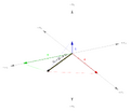 Figure 4. In this dimensionality-3 nullity-1 case, the central 1-parallelotope (a line) occupying all 3 dimensions of tone space projects additional 1-parallelotopes which each occupy 1 of those dimensions; it projects one of these for each combination of 1 dimension from the total 3 (for a total of 3 1-parallelotopes), and each of whose 1D areas (length) corresponds with an entry in the multicomma.
 -
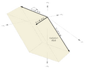 Figure 5a. In this dimensionality-3 nullity-3 case, the central 3-parallelotope (a parallelepiped) occupying all 3 dimensions of tone space projects additional 3-parallelotopes which each occupy 3 (all) of those dimensions; it projects one of these for each combination of 3 dimensions from the total 3 (for a total of 1 3-parallelotope, which is in fact identical to the central 3-parallelotope) and each of whose 3D areas (volume) corresponds with an entry in the multicomma. But this comma basis has not yet been reduced, so it doesn't quite make sense yet.
 -
 Figure 5b. In this dimensionality-3 nullity-3 case, the comma basis has been reduced to reveal that this is a temperament where all intervals are made to vanish. So, space is tiled completely by this periodicity block with only a single pitch inside it.
 -
 Figure 6. In this dimensionality-3 nullity-0 case, the central 0-parallelotope (a point) occupying all 3 dimensions of tone space projects additional 0-parallelotopes which each occupy 0 (none) of those dimensions; it projects one of these for each combination of 0 dimensions from the total 3 (for a total of 0 0-parallelotopes), and each of whose 0D areas (a concept which isn't really defined) corresponds with an entry in the multicomma. So here there are no periodicity blocks, but we can still reach every point in the lattice using the primes themselves; this is JI, since no intervals are made to vanish.


Generator detemperings
Using LA, it is possible to find generator detemperings using the method explained here: Generator detempering#Finding the generator preimage transversal
Using EA, a different method has been found for finding generator detemperings, but it only works for rank-2 temperaments. The method is described with a mathematical lean and accompanying proof here: Wedgies and multivals#How the period and generator falls out of a rank-2 wedgie Some alternatively styled walkthroughs of this method are presented here.
Example 1: full walkthrough
Consider meantone. Here is its multimap, with its indices labelled:
[math]\displaystyle{
\begin{array} {c}
& (2,3) & (2,5) & (3,5) \\
\langle & 1 & 4 & 4 & ]] \\
\end{array}
}[/math]
We only care about the entries whose indices have 2 in them, so that's the first two. We can throw away the remainder:
[math]\displaystyle{
\begin{array} {c}
& (2,3) & (3,5) & \color{red}\cancel{(3,5)} \\
\langle & \color{blue}1 & \color{blue}4 & \color{red}\cancel{4} & ]] \\
\end{array}
}[/math]
We need to know the remaining numbers' greatest common divisor, because that will tell us the period. We don't need this information right away, but we'll use it in a moment. In this case, because one of the numbers is 1, the answer is obvious. We'll look at general ways of finding this later, here: Varianced Exterior Algebra#How to solve the equations.
[math]\displaystyle{ \text{gcd}(\color{blue}1\color{black},\color{blue}4\color{black}) = 1 }[/math]
Let's associate each of these numbers with a variable. How about x and y.
[math]\displaystyle{
\begin{array} {c}
& (2,3) & (3,5) \\
\langle & 1 & 4 & … & ] \\
& \color[rgb]{0,0.666,0}x & \color[rgb]{0,0.666,0}y \\
\end{array}
}[/math]
So now we make each of those numbers into a coefficient on its variable.
[math]\displaystyle{
\begin{array} {c}
& (2,3) & (3,5) \\
\langle & \color{blue}1 & \color{blue}4 & … & ] \\
& \color{blue}1\color{black}x & \color{blue}4\color{black}y \\
\end{array}
}[/math]
And set up an equation where they sum to the period we found in the earlier step to be 1.
[math]\displaystyle{ 1x \color[rgb]{0,0.666,0}+\color{black} 4y \color[rgb]{0,0.666,0}= 1\color{black} }[/math]
Solve. This one's pretty easy to eyeball. Sometimes it won't be though, so we'll come back to a general method for this step in more detail later too (it's actually connected to the method for the GCD calculation). For now the simplest solution that falls out seems to be
[math]\displaystyle{ x=1, y=0 }[/math]
Now this is the clincher: what we do with these results. Let's bring them back with the rest of our info so far.
[math]\displaystyle{
\begin{array} {c}
& (2,3) & & (2,5) \\
\langle & 1 & & 4 & … & ] \\
& 1x & + & 4y & = & 1 \\
& \color[rgb]{0,0.666,0}x=1 & & \color[rgb]{0,0.666,0}y=0 \\
\end{array}
}[/math]
From each compound index, take the other number besides the 2:
[math]\displaystyle{
\begin{array} {c}
& (2,\color{blue}3\color{black}) & & (2,\color{blue}5\color{black}) \\
\langle & 1 & & 4 & … & ] \\
& 1x & + & 4y & = & 1 \\
& x=1 & & y=0 \\
& \color{blue}3 & & \color{blue}5 \\
\end{array}
}[/math]
And now raise those numbers to the xth and xth powers, respectively.
[math]\displaystyle{
\begin{array} {c}
& (2,3) & & (2,5) \\
\langle & 1 & & 4 & … & ] \\
& 1x & + & 4y & = & 1 \\
& \color{blue}x\color{black}=1 & & \color{blue}y\color{black}=0 \\
& 3^{\color{blue}x} & & 5^{\color{blue}y} \\
\end{array}
}[/math]
The product of those powers is a member of our target generator's preimage.
[math]\displaystyle{
\begin{array} {c}
& (2,3) & & (2,5) \\
\langle & 1 & & 4 & … & ] \\
& 1x & + & 4y & = & 1 \\
& x=\color{blue}1 & & y=\color{blue}0 \\
& 3^{\color{blue}1} & \color[rgb]{0,0.666,0}× & 5^{\color{blue}0} & \color[rgb]{0,0.666,0}= & \color[rgb]{0,0.666,0}\frac31 \\
\end{array}
}[/math]
So 3/1 is a valid JI tuning of the generator for meantone, or we could say it's a JI interval the generator approximates.
Because of how this method works, it's clear that it would never be capable of returning any preimage members with factors of 2 in them, so there's no way it could have given us 3/2 or 4/3 straight away. We are likely to need to octave reduce, take the reciprocal, or adjust the result by commas in the temperament. But we've got somewhere to start.
Example 2: simplified
Another example: magic. Slightly abridged this time through, hopefully it's the right amount of info to follow along:
[math]\displaystyle{
\langle\langle 5 \; 1 \; -10 ]] \\
5\;1\\
\text{gcd}(5,1) = 1 \\
5x + 1y = 1 \\
x=0, y=1 \\
3^{0}5^{1} = \frac51 \\
}[/math]
Again, 5/1 is valid, though we usually reduce it to 5/4.
Example 3: higher-dimensionality
This also works for higher-dimensionality temperaments. Each higher dimension adds another variable, which can make it harder to solve. Let's look at septimal meantone:
[math]\displaystyle{
\langle\langle 1 \; 4 \; 10 \; 4 \; 13 \; 12 ]] \\
1\;4\;10\\
\text{gcd}(1,4,10) = 1 \\
1x + 4y + 10z = 1 \\
x=1, y=0, z=0 \\
3^{1}5^{0}7^{0} = \frac31 \\
}[/math]
In that case it was still really easy to solve the equation by eye-balling it. We do still plan to look at a method that works in general here: Varianced Exterior Algebra#How to solve the equations
Why it doesn't work for higher-rank temperaments
So we've seen that the method works for higher-dimensionality temperaments. However, it fails as soon as you try to go higher-rank than 2. The problem arises the step where you select the numbers from the indices that aren't 2. These numbers are to be used as bases for powers of the variables solved for in the previous step. But if there is more than one number in the index besides 2, what could that possibly mean? For example:
[math]\displaystyle{
\langle\langle 1 \; 2 \; -2 \; -5 ]] \\
1\;2\;-2\\
\text{gcd}(1,2,-2) = 1 \\
1x + 2y + -2z = 1 \\
x=1, y=0, z=0 \\
(3,5)^{1}(3,7)^{0}(5,7)^{0} = \; ? \\
}[/math]
We have no way of raising (3, 5) to a power, so the method breaks down.
How to solve the equations
Sometimes the answers to the GCD or the x, y, z, … equations won't fall out for you. In that case you have several options.
In Wolfram Language, the ExtendedGCD[] function will give you everything you need. Consider the example of porcupine, whose first two entries are 3 and 5:
In:  ExtendedGCD[3,5]
Out: {1, {2, -1}}
The first result, 1, is the GCD. The other two results are a solution for x and y:
[math]\displaystyle{ 3x + 5y = 1 \\ 3(2) + 5(-1) = 1 \\ 6 + -5 = 1 \\ }[/math]
So that tells us our generator is 325−1 = 9/5, which is reasonable, though usually taken the reciprocal and octave-reduced to 10/9.
It's also possible to find just the answers to the equations in Wolfram Language using FindInstance[], if you prefer to work it out this way:
In:  3^x*5^y /.First[FindInstance[3x+5y==1,{x,y}, Integers]]
Out: 9/5
Working through the Extended Euclidean Algorithm
To get technical, the solutions to the equations with x and y are Bézout coefficients. They are essentially byproducts of a particular method of calculating the GCD, the Extended Euclidean algorithm, which is why they come bundled in one neat package as part of Wolfram Language's ExtendedGCD[] function. You can work through this method by hand if you'd like to understand it more deeply. At least the case of finding the GCD of just two numbers is fairly easy to work through. Let's try it on the example of porcupine. So we're looking for the GCD of [math]\displaystyle{ \color{Aquamarine}3\color{black} }[/math] and [math]\displaystyle{ \color{Magenta}5\color{black} }[/math].
Begin by finding the [math]\displaystyle{ \color{Orange}\text{remainder} }[/math] after dividing the [math]\displaystyle{ \color{Magenta}\text{bigger} }[/math] of the two numbers by the [math]\displaystyle{ \color{Aquamarine}\text{smaller} }[/math]:
[math]\displaystyle{ \color{Magenta}5\color{black} \bmod \color{Aquamarine}3\color{black} = \;\color{Orange}?\color{black} }[/math]
Or, equivalently, [math]\displaystyle{ \color{Orange}\text{how much you still have to add} }[/math] in order to get the [math]\displaystyle{ \color{Magenta}\text{bigger} }[/math] number after you find how many times the [math]\displaystyle{ \color{Aquamarine}\text{smaller} }[/math] number goes into the bigger one without going over:
[math]\displaystyle{ \color{Magenta}5\color{black} = \;?×\color{Aquamarine}3\color{black}\; + \;\color{Orange}?\color{black} }[/math]
So this value we're looking at is the [math]\displaystyle{ \color{Orange}\text{orange question mark}\color{black} }[/math]. The other [math]\displaystyle{ \text{black question mark} }[/math] is less important now, but we will need it later, and at that time it will be revealed why we needed to rewrite the equation in this more complicated way. So, our solution is:
[math]\displaystyle{ \color{Magenta}5\color{black} = 1×\color{Aquamarine}3\color{black} + \color{Orange}2\color{black} }[/math]
Now we need to recurse the process. Use the colors to follow which numbers went where.
[math]\displaystyle{ \color{Aquamarine}3\color{black} = \;?×\color{Orange}2\color{black}\; + \;\color{YellowGreen}?\color{black} }[/math]
So this time, we still want to find a remainder, but it's the remainder when the [math]\displaystyle{ \color{Orange}\text{previous step's remainder} }[/math] is divided into the [math]\displaystyle{ \color{Aquamarine}\text{previous step's divisor} }[/math]. And so this time we're looking for the [math]\displaystyle{ \color{YellowGreen}\text{green question mark}\color{black} }[/math]. And that gets us:
[math]\displaystyle{ \color{Aquamarine}3\color{black} = 1×\color{Orange}2\color{black}\; + \color{YellowGreen}1\color{black} }[/math]
Recurse again. Now we're looking for the [math]\displaystyle{ \color{Orchid}\text{purple question mark}\color{black} }[/math]:
[math]\displaystyle{ \color{Orange}2\color{black} = \;?×\color{YellowGreen}1\color{black}\; + \;\color{Orchid}?\color{black} }[/math]
And that gives us:
[math]\displaystyle{ \color{Orange}2\color{black} = 2×\color{YellowGreen}1\color{black}\; + \color{Orchid}0\color{black} }[/math]
Upon reaching [math]\displaystyle{ \color{Orchid}0\color{black} }[/math], the recursive process is complete. We've found the GCD: it's the most recent non-zero remainder, which in this case is [math]\displaystyle{ \color{YellowGreen}1\color{black} }[/math].
But what we're really interested in now are those Bézout coefficients! To find these, we just need to work our way backwards through this series of equations we've created. The last equation where we found the [math]\displaystyle{ \color{Orchid}0\color{black} }[/math] is irrelevant now. So beginning with the penultimate one and working backwards, then, our solved equations are:
[math]\displaystyle{ \color{Aquamarine}3\color{black} = 1×\color{Orange}2\color{black}\; + \color{YellowGreen}1\color{black} \\ \color{Magenta}5\color{black} = 1×\color{Aquamarine}3\color{black}\; + \color{Orange}2\color{black} }[/math]
Each of these equations are currently solved for the previous steps' divisor (or in the first case, the [math]\displaystyle{ \color{Magenta}\text{bigger}\color{black} }[/math] of our two original numbers). We're going to rearrange them so that they're solved instead for the remainders.
[math]\displaystyle{ \color{Aquamarine}3\color{black} - 1×\color{Orange}2\color{black} = \color{YellowGreen}1\color{black} \\ \color{Magenta}5\color{black} - 1×\color{Aquamarine}3\color{black} = \color{Orange}2\color{black} }[/math]
Now, we can begin substituting. In the first equation, substitute in for the [math]\displaystyle{ \color{Orange}\text{divisor}\color{black} }[/math] the value it's equal to in the next equation as the [math]\displaystyle{ \color{Orange}\text{remainder}\color{black} }[/math]:
[math]\displaystyle{ \color{Aquamarine}3\color{black} - 1×(\color{Magenta}5\color{black} - 1×\color{Aquamarine}3\color{black}) \;= \color{YellowGreen}1\color{black} }[/math]
Distribute:
[math]\displaystyle{ \color{Aquamarine}3\color{black} - 1×\color{Magenta}5\color{black} + 1×\color{Aquamarine}3\color{black} = \color{YellowGreen}1\color{black} }[/math]
For clarity, we're going to add a black [math]\displaystyle{ 1× }[/math] at the beginning:
[math]\displaystyle{ 1×\color{Aquamarine}3\color{black} - 1×\color{Magenta}5\color{black} + 1×\color{Aquamarine}3\color{black} = \color{YellowGreen}1\color{black} }[/math]
So now it's more obvious how to simplify:
[math]\displaystyle{ 2×\color{Aquamarine}3\color{black} - 1×\color{Magenta}5\color{black} = \color{YellowGreen}1\color{black} }[/math]
And there's our Bézout coefficients, in black! We've gotten 2 and −1 as our answers, just as Wolfram Language found for us above.
Decomposability
When we use the wedge product to wedge together some vectors, the result is a multivector. This multivector can also be said to decompose back into these same vectors. A bivector is a multivector that decomposes into two vectors, a trivector is a multivector that decomposes into three vectors, and so on.
For example, the bivector [[28 -19 12⟩⟩ can be found as the wedge product of the vector [4 -4 1⟩ and the vector [7 0 -3⟩, so it can also be understood to decompose into the set of those two vectors. Its dual is the monocovector ⟨12 19 28], which by virtue of being a monovector is already a vector, or in other words, it doesn't need to be decomposed to be expressed as a set of vectors; it is already a set of one vector.
Just as mappings and comma bases (for temperaments with grade > 1) are not unique, decompositions are not unique. We could also have decomposed [[28 -19 12⟩⟩ into [11 -4 -2⟩ and [-15 8 1⟩, or any other of infinitely many possibilities.
Any multivector found as the wedge product of vectors is decomposable, but not all multivectors are decomposable. If a multivector is chosen at random, for instance, there is no guarantee that it can be decomposed into the wedge product of vectors. Such indecomposable[note 18] multivectors do not represent temperaments. This can be understood through the close relationship between multivectors and matrices in RTT:
- The vectors a multivector decomposes into are equivalent to either the rows of a mapping or the columns of a comma basis, depending on whether the multivector was a multimap or a multicomma, respectively.
- The corresponding multivector is a list of the largest-minors of the matrix.
An indecomposable multivector has no such equivalent matrix which it is the largest-minors for. And indecomposable vectors have no relevance for RTT. These ideas are discussed further in this section: Douglas Blumeyer and Dave Keenan's Intro to exterior algebra for RTT#Possibility of indecomposable varianced multivectors.
Linear dependence between multivectors
Linear dependence is a property defined across bases, i.e. basis vector sets. Multivectors can be understood as vector sets: sets of the vectors they decompose into, and when representing temperaments, these vector sets are understood to be bases.
A quick check for linear dependence between multivectors is to use the wedge product. If the wedge product of two multivectors outputs a multivector whose entries are all zeros, then the input multivectors are linearly dependent; otherwise they are linearly independent.
This method does not give you the actual values of the shared basis vectors, though. Neither does simply decomposing the multivectors individually. If you want to find what these shared basis vectors are, you can convert the multivectors to matrices and use the process described here: Linear dependence#For a given set of basis matrices.2C how to compute a basis for their linearly dependent vectors.
Multivector addition
Entry-wise addition and subtraction works on multivectors in the same way it works for vectors, with simple entry-wise addition: match up entries individually, and add or subtract them (then canonicalize). Vectors are, after all, multivectors themselves: a plain vector is just a multivector with a multiplicity of 1, or in other words, a monovector. In general, we can refer to this approach to temperament addition as multivector addition, which it is also known by outside of xenharmonics.
Let's look an example of a temperament sum performed with EA. So septimal meantone + flattone = godzilla, because:
[math]\displaystyle{ \begin{array} {r} & \langle\langle & 1 & 4 & 10 & 4 & 13 & 12 & ]] \\ + & \langle\langle & 1 & 4 & -9 & 4 & -17 & -32 & ]] \\ \hline & \langle\langle & 2 & 8 & 1 & 8 & -4 & -20 & ]] \\ \end{array} }[/math]
And as for the temperament difference, septimal meantone - flattone = meanmag, because:
[math]\displaystyle{ \begin{array} {r} & \langle\langle & 1 & 4 & 10 & 4 & 13 & 12 & ]] \\ - & \langle\langle & 1 & 4 & -9 & 4 & -17 & -32 & ]] \\ \hline & \langle\langle & 0 & 0 & 19 & 0 & 30 & 44 & ]] \\ \end{array} }[/math]
Exterior powers
Multivector addition may be said to occur in exterior powers of an original vector space. Bivectors live in the second exterior power, trivectors live in the third exterior power, regular vectors are the first exterior power, and scalars live in the zeroth exterior power. Exterior algebra could be said to be all of these exterior powers taken together.
It is even possible to perform temperament addition on multivectors of different grades, although this doesn't have much application for RTT; for example, ⟨16 25 37 45] + ⟨⟨ 1 4 10 4 13 12 ]] is defined, but doesn't simplify to anything giving additional insight. You could think of it like adding x to x².
Advantages of EA
Many of the advantages of EA listed here are things one can do with simple lists of the largest-minors of temperament matrices, i.e. without actually leveraging EA-specific concepts. So we think it's generous but reasonable to collect them here nonetheless.
Pure representation of temperament information
Identifying temperaments by their canonical multimap can be advantageous, because that information is "independent of the choice of generators"[note 19].
Varianced multivectors contain exclusively what we could call "temperament information", without any "generator-size information" as is also present in the case of mapping matrices, or "specific commas information" as is also present in the case of comma bases. In other words, when we consider the canonical mapping for a temperament, while it does effectively uniquely identify a temperament, one does nonetheless have to "look through" the generator-size information that it also contains to see that pure temperament information. And so we could say that varianced multivectors are great from an information architecture standpoint, because they perfectly capture the information about the temperament without any extraneous information, such as whether, say, this is meantone with generators of ~2/1 and ~3/1 or a meantone with generators of ~2/1 and ~3/2.
Temperament addition
It is much easier to perform temperament addition by entry-wise addition of varianced multivectors in EA than it is to do it by matrices in LA. The EA approach is described in a previous section, here: Douglas Blumeyer and Dave Keenan's Intro to exterior algebra for RTT#Multivector addition
With a matrix-based approach, it is necessary to get the matrices into a specific form (with the linearly dependent basis vectors explicitly shared, but also defactored) before entry-wise adding, which is remarkably tricky to do. Furthermore, the only way to check the temperaments' negativity is to essentially convert them to EA form by finding their largest-minors then verifying their leading or trailing entry's sign as described below; this means that while LA can be used to find the temperament sum and difference, if one wants to know which of the two results is the sum and which is the difference, one essentially needs to look at their EA canonical forms.
The only trickiness involved in multivector addition is the computation of the multivector representations of the temperaments in the first place, which is done using the wedge product, which is discussed in detail in this article. And if your temperaments are already represented by multivectors, this is no trickiness at all. Regarding temperament negativity, multimaps with positive leading entries are positive, and otherwise negative; multicommas with positive trailing entries are positive, and otherwise negative.
One way of explaining why doing temperament addition using matrices is so much more complicated than doing it using multivectors is that multivectors are a pure representation of temperament information (as discussed in the previous section). So all the convoluted steps required when doing this for matrices are just what is necessary to get around this extra information and prevent it from obstructing the correct calculation of the temperament-related information.
While multivectors provide you a quick computation of temperament addition, it should also be noted that they conceal how and why temperament addition ever works at all; specifically, you can't see addability (in the sense of the explicit linear-dependence basis constituting all but one of the basis vectors) in a compressed multivector representation in the same way you can see it in the separated vectors listed in the matrix representation. If you are engaged in a temperament addition based exploration, and know what you're doing, then you're already thinking in terms of the underlying basis vector sets, and matrices are the way you would view such decomposed vector sets. So it wouldn't make sense to say that working exclusively in EA would be the better choice for temperament addition, because you couldn't see what you were doing, then; you'd get lost after the first temperament adding. You must keep track of the underlying vector sets as a matrix to keep going. So it would only really be appropriate to say it the other way around: that entry-wise addition of largest-minors is an expedient way to compute your final results, and if you're planning to keep going in one direction or another, then checking the leading/trailing entry of the largest-minors is a necessary check of your temperaments' negativities.
Computing TE complexity
Varianced multivectors can be used as an effective way to compute TE complexity.
The meaning of varianced multivector entries
The entries of varianced multivectors have meaning individually and can provide additional insight into the nature of the temperament they represent. Here we'll look at one way to interpret the entries of the multimap, and one way to interpret the entries of the multicomma.
As we know, the values of the dual varianced multivectors for a given temperament have the same values (just reversed, and with some sign changes), so the important distinction here between the multimap entries and the multicomma entries is: which combination of primes the values are associated with via their compound index. The compound indices contain complementary primes to their corresponding compound index in the dual, but every bit of straightforwardness helps when articulating these things.
So, these two interpretations can be understood as very similar to each other, little more really than restatements of the same general ideas. But one way may click really well for some people, and not for others, so we'll just present it every way we've seen to be helpful at all.[note 20]
Multimap entries: distinct pitch count when prime combination is pitch class equivalent
In an earlier section we looked at how to geometrically visualize the wedge product: Douglas Blumeyer and Dave Keenan's Intro to exterior algebra for RTT#Geometric visualization. It turns out that we can use these visualizations for a bit more than simply understanding the interrelation of the entries of a multicomma. Let's contiue from where that section left off.
So why does it matter how many JI pitches are inside each of these planes defined by particular subsets of primes? Well, each entry of a multimap represents the count of distinct pitches when every prime of its compound index is treated as an equave.
Let's look at this in terms of the multimap for 12-ET. First, the entry with compound index (2) and value of 12. That means that in this temperament (i.e., when both of its commas are made to vanish), and also prime 2 (the octave) has pitch class equivalence, then there are only 12 distinct pitches in the system (we must be mindful that even when rank is 1, that just means there's only one generator, but you can still get infinity pitches from one generator if you don't also apply some sort of pitch class equivalence!). And similarly, if instead prime 3 is what causes pitch class equivalence (i.e. if there's tritave-equivalence instead of octave-equivalence), then there are 19 distinct pitches. And for pentave-equivalence there would be 28.
This might seem underwhelming in the case of this example because we already know, of course, that the multimap ⟨12 19 28] tells us that in this temperament it takes 12 steps to reach the approximation of prime 2, 19 steps to reach the approximation 3, and 28 steps to reach 5. But this conceptualization may become more compelling when we look at it for higher rank temperaments, and the periodicity blocks are higher dimensional.
So let's take a look for a more complex temperament: ⟨⟨ 1 4 10 4 13 12 ]], which is septimal meantone, and which has compound indices of (2,3) (2,5) (2,7) (3,5) (3,7) (5,7). So if we look at the third entry here, that tells us that if we treat both 2 and 7 as having pitch class equivalence, then there are 10 distinct pitches here. Now, we don't usually treat more than one prime at a time as octave equivalent! So if you're in any other rank but 1, that means there are still an infinitude of distinct pitches. It's not until you treat every single prime in the multimap entry's compound index that its value can give you a finite count of distinct pitches—no partial credit!
There may still be some sort of "partial credit" insight here, however, if you, say, only treat 2 as pitch class equivalent, then interrogate the nature of the infinitude of distinct pitches that remain. They come in groups of 10. Each group—well, let's just call it a block, since we know it's a periodicity block—is offset from the next by one factor of 7. So maybe there's some good scales in this tuning with multiples of 10 pitches, i.e. overlaid copies of this 10-block, separated by 7's.
Note that the particular shapes of the periodicity block may also be of interest, as they demonstrate in their offset rows and columns the structure of scales you can build from them.
Multicomma entries: tempered lattice fractions generated by prime combinations
So we now understand how to get to canonical multimaps. And we understand that they uniquely identify the temperament. But what about the individual terms—do they mean anything in and of themselves? It turns out: yes!
The first thing to understand is that each term of the canonical multimap pertains to a different combination of primes. We already know this: it’s how we calculated it from the mapping-row-basis. For example, in the canonical multimap for meantone, ⟨⟨ 1 4 4 ]], the 1 is for (2, 3), the first 4 is for (2, 5), and the second 4 is for (3, 5).
Now, let’s convert every term of the canonical multimap by taking its absolute value and its inverse. In this case, each of our terms is already positive, so that has no effect. But taking the inverse converts us to 1/1, 1/4, 1/4. These values tell us what fraction of the tempered lattice we can generate using the corresponding combination of primes.
What does that mean? Who cares? The motivation here is that it’s a good thing to be able to generate the entire lattice. We may be looking for JI intervals we could use as generators for our temperament, and if so, we need to know what primes to build them out of so that we can make full use of the temperament. So this tells us that if we try to build generators out of primes 2 and 3, we will succeed in generating 1/1 or in other words all of the tempered lattice. Whereas if we try to build the generators out of primes 2 and 5, or 3 and 5, we will fail; we will only be able to generate 1/4 of the lattice. In other words, prime 5 is the bad seed here; it messes things up.
_(2).png)
It’s easy to see why this is the case if you know how to visualize it on the tempered lattice. Let’s start with the happy case: primes 2 and 3. Prime 2 lets us move one step up (or down). Prime 3 lets us move one step right (or left). Clearly, with these two primes, we’d be able to reach any node in the lattice. We could do it with generators 2/1 and 3/1, in the most straightforward case. But we can also do it with 2/1 and 3/2: that just means one generator moves us down and to the right (or the opposite), and the other moves us straight up by one (or the opposite) (see Figure 7). 2/1 and 4/3 works too: one moves us to the left and up two (or… you get the idea) and the other moves us straight up by one. Heck, even 3/2 and 4/3 work; try it yourself.
_(1).png)
But now try it with only 5 and one other of primes 2 or 3. Prime 5 takes you over 4 in both directions. But if you have only prime 2 otherwise, then you can only move up or down from there, so you’ll only cover every fourth vertical line through the tempered lattice. Or if you only had prime 3 otherwise, then you could only move left and right from there, you’d only cover every fourth horizontal line (see Figure 8).
One day you might come across a canonical multimap which has a term equal to zero. If you tried to interpret this term using the information here so far, you'd think it must generate 1/0th of the tempered lattice. That's not easy to visualize or reason about. Does that mean it generates essentially infinity lattices? No, not really. More like the opposite. The question itself is somewhat undefined here. If anything, it's more like that combination of primes generates approximately none of the lattice. Because in this situation, the combination of primes whose canonical multimap term is zero generates so little of the tempered lattice that it's completely missing one entire dimension of it, so it's an infinitesimal amount of it that it generates. For example, the 11-limit temperament 7&12&31 has canonical multimap ⟨0 1 1 4 4 -8 4 4 -12 -16] and mapping-row-basis [⟨1 0 -4 0 -12] ⟨0 1 4 0 8] ⟨0 0 0 1 1]}; we can see from this how primes (2, 3, 5) can only generate a rank-2 cross-section of the full rank-3 lattice, because while 2 and 3 do the trick of generating that rank-2 part (exactly as they do in 5-limit meantone), prime 5 doesn't bring anything to the table here so that's all we get.
Disadvantages of EA
EA is a higher-level mathematical topic
EA is harder to learn and use than LA, and less people know how to use it.
The linearly dependent exception to the wedge product
There is an exception to the wedge product where the result will not give you the same useful temperament you would get by merging using the analogous LA method of concatenating temperament matrices. When two varianced multivectors are linearly dependent, every entry in the resultant wedge product will be 0.
For example, the canonical multimap for 11-limit meantone is ⟨⟨ 1 4 10 18 4 13 25 12 28 16 ]] and the canonical multimap for 11-limit meanpop is ⟨⟨ 1 4 10 -13 4 13 -24 12 -44 71 ]]. We know they share a common basis vector because you can find meantone's multimap as the wedge product of ⟨31 49 72 87 107] and ⟨12 19 28 34 42], and you can find meanpop's multimap as the wedge product of ⟨31 49 72 87 107] and ⟨19 30 44 53 66]; the basis vector shared in common is ⟨31 49 72 87 107]. So, wedging ⟨⟨ 1 4 10 18 4 13 25 12 28 16 ]] and ⟨⟨ 1 4 10 -13 4 13 -24 12 -44 71 ]] won't give something useful, as you might expect! Normally, wedging two 5-D bicovectors would give a 5-D quadricovector representing another temperament. But in this case we get ⟨⟨⟨⟨ 0 0 0 0 0 ]]]]. Note that you can still map-merge these temperaments using the linear algebra method—by concatenating their mappings and reducing—just fine. That looks like:
map-merge([⟨1 0 -4 -13 -25] ⟨0 1 4 10 18]}, [⟨1 0 -4 -13 24] ⟨0 1 4 10 -13]}) = [⟨1 0 -4 -13 0] ⟨0 1 4 10 0] ⟨0 0 0 0 1]}
and if you wedge together those three covectors you get the tricovector for this temperament, ⟨⟨⟨ 0 0 1 0 4 10 0 4 13 12 ]]], which is called erato, that the wedge product was unable to provide for us. Well, it can, but only if you remove the shared vector from all but one of the wedged multimaps; e.g. removing 31 from one or the other and doing meantone∧19 or meanpop∧12 will work.
There is an argument that because this aspect of EA means that the wedge product can be used for a quick check of linearly dependence, that constitutes an advantage to EA. But surely its nonconformity with the results of the simpler LA on the matter of temperament merging is a much more major detractor. Especially when it's not difficult to check for linearly dependence in LA either (concat matrices, HNF, see if there are any zero-rows).
How to think about why it's different in EA
To understand why this happens, it may help to review the geometric visualization of the wedge product described earlier Douglas Blumeyer and Dave Keenan's Intro to exterior algebra for RTT#Geometric visualization, which shows how the wedge product of two vectors is the paralellogram formed from these vectors as its sides. If the two input vectors were linearly dependent (and if they are monovectors the only way this could be would be if they were the same vector or a multiple of it!) then of course the area would be 0. In this case we are indeed looking for a standard 2-D area, because the grade of this result is 1 + 1 = 2. In other words, even the wedge product of two linearly dependent monovectors is a bivector.
Now let's think about the example of wedging a monovector with a bivector. Assuming linear independence, the resulting shape will be a parallelepiped, i.e. a higher dimensional parallelogram. Basically if the bivector is that paralellogram we described connecting points O, A, B, and AB, and the monovector is from O to C, then we need to create two new parallelograms: one between C and A in the same way we made one between A and B, and also one between C and B. But then we'll only have half of our parallelepiped. Like a cube it has 6 faces but these are only 3 of those 6—the three which touch the vertex O. So each of these parallelograms needs a copy on the opposite side (in the same way that in the simpler case we needed a copy of A opposite the first A, and a copy of B opposite the first B, to close the shape). And so, the wedge product of this monovector and bivector is a trivector which represents the 3-D area—or volume as we typically call this dimensionality of area—of this resulting parallelepiped.
But now what if we wedged a monovector with a bivector, but they were linearly dependent? This means that our monovector from O to C is not in a new direction, but a point along the same trajectory as either A or B. That means that the resulting parallelepiped is going to be just the same parallelogram that we had already from A and B! However, we have increased the grade from 2 to 3 by wedging with this monovector, so now, instead of asking for the 2-D area of this parallelogram, which has a positive value, we're asking for its 3-D area, and of course a 2-D shape has no 3-D area. So that's why we get zeros here.
This principle gets more difficult to imagine beyond the 3-D realm that we inhabit as physical beings, but hopefully if the limitation makes sense this far, you can accept the abstraction.
The varianced multivector format lacks direct information about dimensionality
When we consider a matrix-based representation of a temperament, such as a mapping, we have near-immediate access to three key pieces of information about the temperament:
- the rank (r)
- the dimensionality (d)
- the nullity (n)
As an example, consider meantone temperament's mapping: [⟨1 0 -4] ⟨0 1 4]}. We can get the rank from the row count: 2. We can get the dimensionality from the column count: 3. And we can get the nullity from the rank–nullity theorem, which essentially states that r + n = d. So nullity should be 1. We can equivalently get this information from meantone's comma basis [[4 -4 1⟩]; the nullity is the column count, 1, the dimension is the row count, 3, and rank is the difference, 2.
On the other hand, the varianced multivector form of meantone ⟨⟨ 1 4 4 ]] only provides one of these three pieces of information: the rank, which is the count of brackets it's enclosed within. Finding the dimensionality is possible, but involves cross-referencing the count of entries in the largest-minors list with the bracket count in a Pascal's triangle table such as the one demonstrating sign patterns for the EA dual above. Either that, or memorizing sections of Pascal's triangle. And without the dimensionality, the nullity cannot be ascertained from the rank.
For nilovectors, the varianced multivector format also lacks information about variance
Consider the nilovector 1. Without any angle brackets, it is unable to convey which side of duality it is on. So here we have no information about dimensionality or variance.
Compare this situation with the equivalent LA structure, a matrix consisting only of a row or column of zeros. A rank-0 mapping or "zero mapping" looks like [⟨0 0 0…]}, a single row of zeros, structured in the same way as any other mapping, like meantone [⟨1 0 -4] ⟨0 1 4]}. While a zero comma basis looks the other way around, [[0 0 0…⟩], a single column of zeros, structured in the same way as any other comma basis, like meantone [[4 -4 1⟩].
Inefficiency of representing temperaments
While varianced multivectors are indeed compressed forms of tensors (as discussed earlier here), they are not generally smaller in size than a corresponding matrix representation of the same temperament information. In fact, it is only in the case of dimensionality 4 and grade 2 that matrices cannot represent a temperament more succinctly than a varianced multivector, because either the mapping or the comma basis would require 8 total entries (2×4 or 4×2) while the varianced multivector can accomplish this in 6 entries. Everywhere else, matrices are either tied with multivectors or have fewer entries. To be absolutely clear, this comparison allows for using comma bases to specify temperaments when they can do it in fewer entries, despite the fact that the matrix-based canonical form for temperaments is the mapping.
| Matrices | d | Varianced multivectors | d | |||||||||||||||
|---|---|---|---|---|---|---|---|---|---|---|---|---|---|---|---|---|---|---|
| 2 | 3 | 4 | 5 | 6 | 7 | 8 | 2 | 3 | 4 | 5 | 6 | 7 | 8 | |||||
| g | 1 | 2 | 3 | 4 | 5 | 6 | 7 | 8 | g | 1 | 2 | 3 | 4 | 5 | 6 | 7 | 8 | |
| 2 | 3 | 8 | 10 | 12 | 14 | 16 | 2 | 3 | 6 | 10 | 15 | 21 | 28 | |||||
| 3 | 4 | 10 | 18 | 21 | 24 | 3 | 4 | 10 | 20 | 35 | 56 | |||||||
| 4 | 5 | 12 | 21 | 32 | 4 | 5 | 15 | 35 | 70 | |||||||||
| 5 | 6 | 14 | 24 | 5 | 6 | 21 | 56 | |||||||||||
| 6 | 7 | 16 | 6 | 7 | 28 | |||||||||||||
| 7 | 8 | 7 | 8 | |||||||||||||||
For an example of the only case where EA is more efficient, septimal meantone can be represented with the multimap ⟨⟨ 1 4 10 4 13 12 ]] or multicomma [[12 -13 4 10 -4 1⟩⟩, either of which have 6 entries, but its mapping [⟨1 0 -4 -13] ⟨0 1 4 10]} and comma basis [[4 -4 1 0⟩ [13 -10 0 1⟩] require 8 entries.
For an example where they are tied, consider (5-limit) meantone. Whenever rank or nullity are 1, you are guaranteed to have a varianced multivector which is the same size as a matrix; in this case it's the multicomma, [4 -4 1⟩, which is essentially the same as the comma basis [[4 -4 1⟩]. Of course meantone's mapping [⟨1 0 -4] ⟨0 1 4]} has more entries, but what is of interest here is the minimum required entries for a structure in the given algebra to completely identify the object.
And for an example where EA is less efficient, consider the 17-limit, rank-3 temperament represented by the mapping [⟨1 0 0 -5 -13 21 12] ⟨0 1 0 2 6 -8 -5] ⟨0 0 1 2 3 -2 0]}. That's a total of 21 entries, which is a lot. But its corresponding multimap is ⟨⟨⟨ 1 2 3 -2 0 -2 -6 8 5 -6 12 10 12 15 -10 -5 -13 21 12 -11 32 24 37 36 -24 -4 -2 1 -22 -7 -9 -30 -17 -16 -41 ]]], which has 35 entries, and due to being presented as a single unbroken string of numbers, is arguably much harder to read and understand.
To be fair, there is an the argument that 7-limit, rank-2 temperaments as a category are more popular than all 13-limit and higher temperaments with grade ranging from 2 to d-2 combined, or in other words, that the single green cell in the left half of the above table outweighs all of the green cells in the right half of the table, including imagining extending the table off to infinity.
Possibility of indecomposable varianced multivectors
Of course one must at least take care to make sure the count of largest-minors in the list is possible given the grade (rank or nullity, i.e. count of brackets), requiring a similar lookup in a Pascal's triangle as was discussed a couple subsections ago. The only way to mess up a matrix in this way would be to fail to make it rectangular, i.e. fail to make sure that all rows are the same length as each other and all columns are the same length as each other.
But it's actually much more difficult than meeting that straightforward constraint. Consider this varianced multivector, for example, which was randomly generated: ⟨⟨ 2 -4 8 -9 7 2 ]]. As a varianced multivector with grade 2, six is a valid count of largest-minors, because that would pin it at dimensionality 4, so we can see that much is fine; that's not the problem. The problem is that if you try to find a mapping for which this is its list of largest-minors, you will find yourself unable to. This is therefore a "indecomposable" varianced multivector, which can not represent a temperament.
On the other hand, it is not possible to create RTT matrices that don't represent temperaments. They may be completely ridiculous musically, but mathematically they will always be sound.
The reason why it's possible to create indecomposable varianced multivectors this way is because they are a compressed form of temperament information, while matrices are not. Each entry in an RTT matrix is independent. But most varianced multivectors' entries represent the results of interactions between entries in RTT mappings. And it is certainly possible to produce a string of supposed varianced multivector entries which could never all together at once have been the results of a real matrix.
An interesting consequence of this problem is that EA cannot deliver on a promise of easier canonicalization than LA that it might otherwise have had. Canonicalization relies on defactoring, and defactoring in LA is hard; defactoring algorithms are fairly tricky to get your head around. Defactoring in EA is super easy, though: it's just GCD removal and positive leading entry normalization. However, because of the fact that a given varianced multivector cannot be assumed to be decomposable, it must be checked essentially by attempting to decompose it into vectors, which is the equiivalent to converting it to matrix form and back, thus rendering any potential benefits of EA here moot.
Lack of intuitiveness
One can imagine handcrafting RTT mappings directly. The meantone mapping directly speaks to us: give me a world where one of the first generator gets me to prime 2, one of the second generator gets me to prime 3, and prime 5 is gotten to by going down four of the first generator and up four of the second. But the entries of varianced multivectors do not provide this level of direct insight into the functioning of the temperament they represent. The "advantage" discussed in the previous section—"tempered lattice fractions generated by prime combinations"—is not nearly as valuable as the information that mapping entries convey.
Lack of use for tuning
With mappings, reasonable tuning calculations for temperaments are a function away, such as by leveraging the power of the Moore-Penrose inverse function. No such trick exists for varianced multivectors and tuning.
Similarly, generator detemperings can be found from a mapping with the method (described here: Generator detempering#Finding the generator preimage transversal), whereas the method for finding these from multimaps only works for rank-2 (described here: Wedgies and multivals#How the period and generator falls out of a rank-2 wedgie).
Lack of ability to directly change domain basis
As far as this author knows, it is an unsolved problem how to directly change the domain basis for a varianced multivector. At present, they must be converted to matrix form, basis changed, and then converted back.
Summary diagrams and tables

| Terminology category |
Building block → | Temperament ID | EA temperament ID | EA temperament ID dual | Temperament ID dual | ← Building block |
|---|---|---|---|---|---|---|
| RTT application | Map, mapping-row (often an ET) |
Mapping, mapping-row-basis |
Multimap | Multicomma | Comma basis | Interval, comma |
| RTT structure | Map | List of maps | List of largest-minors | list of largest-minors | List of prime-count lists | Prime-count list |
| Linear algebra structure | Row vector, matrix row, covector |
Matrix, list of covectors | Largest-minors row vector, multicovector |
Largest-minors (column) vector, multivector |
Matrix, list of vectors | (Column) vector, matrix column, vector |
| Extended bra-ket notation representation |
Bra | Ket of bras | Nested bras | Nested kets | Bra of kets | Ket |
| RTT jargon | Val | List of vals | Wedgie, multival | Multimonzo | List of monzos | Monzo |
Footnotes
- ↑ You may also see it as geometric algebra which is a superset of EA, or Grassman algebra, which is a synonym. Clifford algebra is also related, but is even more general still.
- ↑ See https://web.archive.org/web/19991109013427/http://cix.co.uk/~gbreed/meantone.htm and https://web.archive.org/web/19991109001944/http://www.cix.co.uk/~gbreed/matrices.htm for examples of RTT matrices from 1999.
- ↑ Gene's earliest posts to Yahoo Groups about wedge products appear to date from November 2001: https://yahootuninggroupsultimatebackup.github.io/tuning-math/topicId_1543.html
- ↑ Unlike tri-, bi-, mono-, the nilo- prefix is not commonplace, but a coinage Dave Keenan and Douglas Blumeyer decided upon for discussions of EA in RTT. The suggested pronunciation of "nilo" is /'nɪ lo/, i.e. to rhyme with "pillow", because other pronunciations might suggest an annihilating covector, i.e. a covector that maps vectors to the null vector. "Nil-" was also considered, but it was felt that, in the case of a nilcovector it would too strongly suggest a (mono) covector with all of its entries equal to 0. Also, nilo- favorably rhymes with mono-.
- ↑ This notation was originally proposed by Dave Keenan here: https://yahootuninggroupsultimatebackup.github.io/tuning-math/topicId_7525#7749
- ↑ Dave Keenan and Douglas Blumeyer also considered the term "vectoral". This noun (emphasis on the first syllable) was coined by them with the etymology of "vector-like thing", by analogy with the nouns "functional" and "orbital". This could have worked both in natural and computer language. But, sensitive about introducing new made-up terminology, they decided not to recommend it.
Note that in RTT with linear algebra, we do not have a need for the generic word for covector and vector, because we do not represent temperaments directly with those objects, so there "vector" is perfectly fine as short for "contravector". - ↑ There's an argument that true "nilocovectors" or "nilovectors" could not exist, because varianced multivectors with grade 0 are neither covariant nor contravariant (their entries vary neither with nor against the units), and therefore that we should only use the generic "nilovector", but we think it is still a good idea to permit both "nilocovector" and "nilocontravector" because they allow you to be specific about on which side of duality you find this object, i.e. it helps you understand its dual in the given temperament.
- ↑ The multilinear algebra from which RTT draws is closely related to "tensor analysis", but not to "tensor algebra", the former being the way that physicists use tensors, while the latter is how general mathematicians use them.
- ↑ or as you might say in MLA, its "indices"
- ↑ We (Dave and Douglas) prepared this article during a period of deep study of Gene's work on RTT, and before we had begun planning to assemble the entire series of articles on RTT which we have started by now. As with the articles in that series, we use our recommended terminology here, terminology which differs from the choices made on other mathematical theory pages. Having a particular interest in this topic, Mike Battaglia contributed to this article as well, and at that time we offered to let him change some of the terminology to match the rest of the mathematical pages (e.g. "multival" instead of "multimap"), but he ultimately decided not to, feeling that while our interpretation and philosophy are different than his, the article remained as it was an excellent read with some helpful information for those learning about exterior algebra. Now that our article series is well on its way, we're unlikely to shift terminology at this point.
- ↑ Most varianced multivectors' dimensionalities are inferable from their grades and entry lists, however, not so for nilovectors; so, for parity with matrices, the dimensionality is required as a fourth entry in their case.
- ↑ If it helps you, you could think of this sign-changing step as paired with the GCD removal step, if you think of it like dividing out a GCD of −1.
- ↑ Or do an anti-transpose sandwich, if you want to be consistent with the process for the dual in linear algebra, as discussed here; either way will work here.
- ↑ The bra-ket notation comes from physics, specifically quantum mechanics.
- ↑ and we could even get a sixth 'p' out of it if we attributed them to Paul Erlich, since he was the person who brought them to our awareness
- ↑ The word "progressive" refers to the fact that it produces parallelotopes of progressively higher "dimensionality" or grade (assuming the inputs are linearly independent).
- ↑ The area of the central parallelotope is of less interest, but can be found as the norm of this multicomma, specifically its "root sum squared": √(12² + 19² + 28²) = √1289 ≈ 35.9.
- ↑ EA has degrees of decomposability; it uses the term "rank" too, but in a completely different sense than how it is used in linear algebra (see here). In EA, rank refers to the degree of decomposability of a multivector, with respect to multivector addition. If a multivector can be decomposed into a wedge product of vectors, then it is rank-1. If a multivector cannot be thus decomposed, however it can be expressed as the entry-wise sum or difference of rank-1 multivectors, then it is higher rank. It's rank is the minimum count of rank-1 multivectors it can be expressed as the sum of.
For example, porcupine plus meantone is tetracot, or ⟨⟨ 3 5 1 ]] + ⟨⟨ 1 4 4 ]] = ⟨⟨ 4 9 5 ]]. We know that porcupine and meantone are each rank-1, because they can be decomposed into wedge products of vectors (⟨1 0 -4]∧⟨0 1 4] and ⟨1 2 3]∧⟨0 3 5], respectively). And in this case, tetracot can also be decomposed into a wedge product of vectors, ⟨1 1 1]∧⟨0 4 9]. So it is possible for two rank-1's to sum to a rank-1. This is because porcupine and meantone differ by only a single vector, or in other words, we can find vector decompositions for these two temperaments that are identical except for one vector. In this case, the shared basis vector would be the map for 7-ET, ⟨7 11 16], and then porcupine and meantone each have one other vector that differs from the additional vector for the other.
An example of a rank-2 multivector is ⟨⟨ 1 9 10 12 13 -2 ]], which is found as the sum of septimal meantone ⟨⟨ 1 4 10 4 13 12 ]] and septimal mavila ⟨⟨ 0 5 0 8 0 -14 ]]. The addends are each decomposable, AKA rank-1. But their sum is indecomposable. We can check this by using any of the multivector-to-matrix methods described in this article, and they will all fail. These two temperaments are not addable because they do not share all but one basis vector; in fact they share no basis vectors, so they aren't linearly dependent. - ↑ Quote from Graham Breed.
- ↑ Here's another way, from Gene himself: https://yahootuninggroupsultimatebackup.github.io/tuning-math/topicId_8953#8953%20Gene%20quote%20about%20numbers%20in%20wedgies%20probably%20add%20it%20to%20EA%20article%20on%20wiki