User:Sintel/Validation of common consonance measures
Many models exist that attempt to give some measure of consonance or dissonance for intervals. However, as far as I am aware, there is very little work on empirically validating these models. Using a dataset of consonance ratings for common just intervals, I will try to find out which of these measures best predicts our perception of consonance.
Data
The data comes from Masina et al. "Dyad's consonance and dissonance".[1]
In their test, subjects rated the consonance of 38 just intervals. They use a harmonic timbre with 10 harmonics, with amplitudes proportional to 1/n, with exponential decays mimicking a plucked string. Each participant was asked to rate the consonance of simultaneous intervals on a 1 to 5 point scale: very dissonant, mildly dissonant, not dissonant nor consonant, mildly consonant, very consonant. These ratings were then normalized to the range (0, 1).
I like this dataset for a few reasons:
- It contains many interesting just intervals (such as 33/32). Most studies only use intervals from 12 equal-temperament.
- It has a wide range of intervals, spanning 2 octaves.
- They did not ask participants to rate the pleasantness, as many other papers do:
To minimize the impact of cultural familiarity, we emphasized not to use the subjective categories of pleasant/unpleasant and familiar/unfamiliar, but rather to judge about the (in principle more objective) degree of unity/division of the sound stimulus, namely whether the two sounds are perceived to mix well together or not.

Note that the unison (1/1) was not included in the test.
Models
Here I will give a brief overview of the models I included for evaluation.
Complexity measures
It is widely accepted that simple (i.e. having small numbers) just intervals are consonant. This motivates the various definition of complexity. There are many models for measuring the complexity of just intervals. Here, I will consider three common ones: the Tenney, Weil, and Wilson norms.
For a ratio n/d in lowest terms:
- Tenney norm is given by [math]\displaystyle{ \log_2(n \cdot d) }[/math]. This gives [math]\displaystyle{ \text{Tenney}\left(\tfrac{15}{8}\right) = \log_2(15 \cdot 8) = 6.90 }[/math].
- The Weil norm is given [math]\displaystyle{ \log_2(\max (n, d)) }[/math]. We have [math]\displaystyle{ \text{Weil}\left(\tfrac{15}{8}\right) = \log_2(15) = 3.91 }[/math].
- The Wilson norm is the sum of prime factors (with repetition). That gives [math]\displaystyle{ \text{Wilson}\left(\tfrac{15}{8}\right) = 5 + 3 + 2 + 2 + 2 = 14 }[/math].
I have also included Euler's gradus suavitatis,[2] which is probably the first complexity measure historically. It is somewhat similar to the Wilson norm, in that it depends on the prime factorization. Given s, the sum of prime factors, and n the number of prime factors, Euler's gradus function is s - n + 1. For example [math]\displaystyle{ \text{Gradus}\left(\tfrac{15}{8}\right) = 14 - 5 + 1 = 10 }[/math].
Roughness
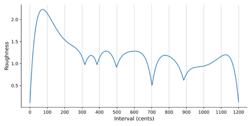
The auditory roughness theory states that dissonance is the result of beating between overtones. First proposed by Helmholtz, these models are quite popular in the psychoacoustics literature, and many variations have been developed over the years. Here, I will use the classic roughness curve as derived by Plomp and Levelt in 1965.[3]

Harmonic entropy
Harmonic entropy is a probabilistic model that measures the degree of uncertainty in the perception of a virtual root. Briefly, it assumes the auditory system tries to fit a harmonic series to the overtones of the incoming dyad. Since there is ambiguity in this process, a set of probabilities is constructed for all possible ratios. The entropy of this distribution then gives a mathematical measure of uncertainty. See the harmonic entropy article for a detailed derivation.
I will use the 'default' parameters, with s = 17 ¢ and [math]\displaystyle{ \sqrt{n \cdot d} }[/math] weights.
Common practice
In common practice Western theory, consonance is usually given as a binary distinction: an interval is either a consonance or a dissonance.
The intervals included as consonances are the unison (1/1), the octave (2/1), the perfect fifth (3/2) and fourth (4/3), the major and minor thirds (5/4 and 6/5), as well as their octave complements (sixths) and their compound intervals (perfect 12th etc.) All other intervals are considered dissonances. This is modeled using simple binary coding, dissonances get a value of 0, consonances a value of 1.
Of course, this is an oversimplified model, since it doesn't even distinguish between perfect and imperfect consonances. It is primarily included to serve as a reasonable baseline.
Results
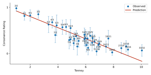
To validate these measures, a linear model was fitted to the perceptual data, using weighted least squares to account for the variance. Since all models have only two parameters (slope and intercept), we can directly compare their R-squared coefficient, which measures how well the model correlates with the data.
| Measure | R2 |
|---|---|
| Tenney | 0.888 |
| Wilson | 0.862 |
| Weil | 0.812 |
| Harmonic entropy | 0.807 |
| Euler gradus | 0.797 |
| Common practice | 0.743 |
| Roughness | 0.742 |
As expected, all models under consideration are reasonably good at fitting the data, and all of them are statistically significant (F-test p < 0.001 for all measures). However, it is clear that the complexities (except for Euler's gradus) do a better job than the rather complicated roughness and harmonic entropy models. Perhaps surprisingly, roughness does worse than the somewhat over-simplified common practice model.
To check for statistical significance, a bootstrapping procedure was followed, giving a sample estimate of the R-squared values. Since Tenney was the best performing model, I compared against all the other measures. Tenney complexity performed significantly better than Weil (p = 0.002), common practice (p = 0.019) and roughness (p = 0.022). It was not significantly better than the other measures.

Continuous extension of the Tenney norm
The strong performance of the Tenney complexity suggests it is quite effective for predicting consonance perception.
However, all complexity models have two serious drawbacks in practice. First, they are only defined for just intervals, making them unable to predict consonance for tempered intervals. Second, they do not take into account the proximity of some complex intervals to simpler ones. To give a simple example, an interval such as 301/200 is very complex, and thus will be predicted as extremely dissonant. In reality, it sounds rather smooth, due to its proximity to 3/2.
Here I propose a continuous extension that preserves the measure's desirable properties while extending it to all possible frequency ratios.
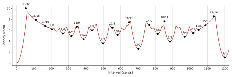
To construct this continuous Tenney measure, we first take a representative set of relatively simple just intervals. The set considered here consists of all intervals with a Tenney norm < 10. Then, take the minimum of a set of parabolas, each reaching its a minimum at one of these ratios, with a value given by the Tenney norm.
More formally, for an interval r in logarithmic units, the continuous Tenney measure is defined:
- [math]\displaystyle{ \text{T}_c(r) = \min_{i} \left\{ \text{Tenney}\left(\frac{n_i}{d_i}\right) + \left(\frac{r - \log_2\frac{n_i}{d_i}}{k} \right)^2 \right\} \, , }[/math]
where [math]\displaystyle{ \tfrac{n_i}{d_i} }[/math] are the just intervals from our representative set, and k is a scaling factor determining the width of the parabolas. k controls how quickly the measure increases as we move away from simple ratios. It roughly corresponds the the amount of tolerance we allow when we consider an interval as approximating a just interval close by. I will use k = 20 ¢. This parameter was not optimized on the current dataset, as doing so would give this measure an unfair advantage over the other models, which use their standard parameters. Note that increasing the set of intervals to a higher cutoff does not change the curve, since it already reaches a maximum below a Tenney norm of 10.

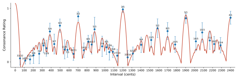
A linear model was then estimated as for the other measures. The continuous Tenney measure resulted in an R-squared value of 0.944, making it the best model so far. At least for this dataset, the difference between this extension and the original Tenney norm is rather small. Despite this, it performed significantly better than all other measures, likely because of the increased accuracy for a few of the more complex ratios.

Discussion
There are various limitations to this analysis. While the participants had varying ages and musical education, they all presumably come from a Western background. As with any psychoacoustic test, the variance in responses was rather large, limiting the statistical power. A larger selection of intervals, especially measuring some more complex ratios, as well as various tempered intervals would be quite valuable for giving some finer distinctions (e.g. comparing Wilson versus Tenney norms). These conclusions are of course only valid for harmonic spectra, and are limited only to dyads.
It is quite clear from the results that models like harmonic entropy, while mathematically sophisticated, do not really improve on 'naive' measures like the Tenney norm. At least for relatively simple ratios (Tenney norm < 10), complexity correlates with perceived dissonance quite well. For more complex intervals, the effect of proximity needs to be taken into account, which can be accomplished using the proposed continuous extension. Practically, the findings suggest that if we want to prioritize certain intervals or give an estimate of consonance, we are better off using complexity rather than roughness or harmonic entropy.
Code availability
All figures and models presented here can be replicated by running the notebook available at: https://gist.github.com/Sin-tel/59ea5446a90119c4bfe5467f4198c9b5.
References
- ↑ I. Masina, G. Lo Presti & D. Stanzial (2022) Dyad’s consonance and dissonance: combining the compactness and roughness approaches. Eur. Phys. J. Plus 137, 1254.
- ↑ Leonhard Euler (1739) Tentamen novae theoriae musicae (Attempt at a New Theory of Music), St. Petersburg.
- ↑ R. Plomp, W. J. M. Levelt (1965) Tonal Consonance and Critical Bandwidth. J. Acoust. Soc. Am.