Cross-domain temperament merging

It is possible to merge regular temperaments that are defined in separate domains.

Steps

1. Determine the domain basis for the output temperament

A guiding principle when performing a temperament merge across domains is described on the main page for temperament merging:

Map-merging produces a temperament that makes to vanish only the commas that are made to vanish by all of the input temperaments.
Conversely, comma-merging produces a temperament that makes to vanish every comma that is made to vanish by any of the input temperaments.

From this, we can make some helpful statements:

For a comma-merge, because the output temperament deals with every comma, then its domain basis must be capable of supporting this: specifically, it must include every basis element from any of the input temperaments' domain bases. Think of it this way: for any given temperament, its domain basis elements are the building blocks for its commas, and so in order to express every comma in the merged temperament, we will need every input temperament's building blocks gathered in one place. In other words, we must find the merge of all the input domain bases.

For a map-merge, then, because the output temperament will deal only with tempered commas shared by every input temperament, then its domain basis only needs to include the basis elements that are present in all of the input domain bases. Here's why: a comma built using a basis element that isn't shared by all input temperaments couldn't even be built in all input temperaments, let alone made to vanish by all of them. And so, to build the set of commas that are made to vanish by all temperaments, we only need the building blocks that can be found in all of them. In mathematical terms, we must find the intersection of the input domain bases.

• 

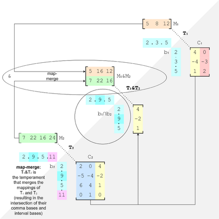  A map-merge across domain bases gives a comma-intersection and a domain basis intersection (for purposes of illustrating this concept, the results are not being canonicalized).

• 

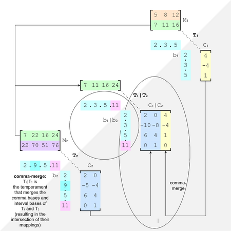  A comma-merge across domain bases gives a map-intersection and a domain basis merge (for purposes of illustrating this concept, the results are not being canonicalized).

2. Convert the input temperaments to the output domain basis

After determining the target domain basis, follow the instructions described here to convert the input temperament over: Cross-domain temperament merging#Changing basis.

3. Perform the merge as usual

See the instructions described here to perform the temperament merge: Temperament merging#Merging.

Domains as subspaces of other domains

In the same way that an subspace is a part of the full space, a subspace can be seen as a part of another larger subspace. So we can say a domain is itself a subspace of another domain.

Any given domain will be a subspace of infinitely many other domains.

Examples

Figure 1. The domain 2.3 can be clearly seen to be a subspace of 2.3.7. The latter is simply many copies of the former, separated by 7's.

For example, the 2.3 domain is a subspace of the 2.3.7 domain; this is clearly apparent, because the 2.3.7 domain is the same as the 2.3 domain except with the addition of a new basis element, 7 (see Figure 1).

Figure 2. Here we can see how the domain 2.9 is a subspace of 2.3. The latter is simply two copies of the former, offset by 3.

For a perhaps less obvious example, the 2.9.5 domain is a subspace of the 2.3.5 domain; this may be surprising, because 2.9.5 is the one with a larger basis element, but what this actually means is that it spans a smaller subspace, because while 2.3.5 contains all intervals with any power of 3, 2.9.5 contains only half of those, specifically those with even powers of 3, i.e., powers of 9 (see Figure 2).

Sometimes, neither domain is a subspace of the other. Consider 2.3.5 and 2.3.7: the former lacks a 7, and the latter lacks a 5.

Application: determining whether it is possible to change the domain

Understanding which domains are subspaces of each other is important when changing the domain for an interval or temperament. This is because only certain changes are possible: specifically, it is only possible to change between domains where one is a subspace of the other. Otherwise, the domains are incomparable.

We then have further constraints, depending on which type of object we're changing the domain for:

• For objects that are made of intervals — such as individual intervals themselves, or comma bases — we can only change in the direction from the subspace to the superspace. This is because unless the target domain completely contains the original domain, there's no guarantee that we'll still have all the basis element building blocks that we need to represent our intervals.
• For objects that are made of maps, i.e. mappings, the opposite is true: we can only change from the superspace to the subspace. Think of it this way: maps are functions, and they only claim to know what to do with inputs from within their given domain, and their domain is the domain. So we can restrict their behavior just fine, because there's no question about what they do with inputs that don't happen to use every available building block from their domain. But there's no unambiguous way to say what they should do with any inputs that use building blocks from outside that domain, if we were to try to expand it.

These two types of objects are in fact the only two types of objects we need to worry about in RTT. The technical term for the difference between these two types of objects is variance. There are only two variances: contravariant, and covariant. Intervals are contravariant, and maps are covariant.

So from these two opposing bulleted facts above, we can conclude that for any pair of domains where neither one is a subspace of the other, there would be no way for us to express either intervals or maps from one in the other. And that's why we could say that they're incomparable domains.

Notably, there is still a way to get intervals to a subspace, and maps to a superspace, but it's indirect. To do so, take the dual of your object, then change basis, then take the dual again. So for a mapping you would use the nullspace function to convert it to its corresponding comma basis, change domain basis, and then use the antinullspace function to convert it back to its corresponding mapping on the other side.

General method to determine whether a domain is a subspace of another

A couple subsections ago, we provided a couple examples where we used natural language to explain — between two domains — which one was a subspace of the other. But we still need to describe a method to determine this in general. Let's do that next.

We can say that a domain with basis [math]B_1[/math] is a subspace of another domain with basis [math]B_2[/math] if when we merge [math]B_1[/math] and [math]B_2[/math] we just get [math]B_2[/math] again. In layperson's terms, if [math]B_1[/math] brings nothing to the table that [math]B_2[/math] hasn't already brought, then it is completely contained by [math]B_2[/math] and therefore is a subspace of it.

For more information on merging domain bases, see Cross-domain temperament merging#Merging.

Example

For instance, we can demonstrate how 2.25/9.11/7 is a subspace of 2.5/3.7.11 using this approach. If you've really got a knack for this stuff, you may be able to eyeball even this somewhat intense example, but it's obviously good to have a rigorous method like this to fall back on, if only to convince ourselves that we've got the right answer (or to automate things with code, as has been done with these methods in the RTT library in Wolfram Language).

So, first, we do the first step of merging domain bases: concatenate them. That gets us 2.25/9.11/7.2.5/3.7.11.

The next step of merging is to canonicalize. To begin that, we represent our basis as a matrix, naturally called our basis matrix [math]B[/math]. Here, we've labeled the columns with the number-list representation of the basis elements, to help show the correspondence, as well as the rows with the primes these basis elements factor into:

[math] \begin{array} {ccc} \begin{array} {ccc} \\ \end{array} \\ \begin{array} {rrr} \scriptsize{2} \\ \scriptsize{3} \\ \scriptsize{5} \\ \scriptsize{7} \\ \scriptsize{11} \\ \end{array} \\ \end{array} \begin{array} {ccc} \begin{array} {ccc} \scriptsize{2} & \scriptsize{25/9} & \scriptsize{11/7} & \scriptsize{2} & \scriptsize{5/3} & \scriptsize{7} & \scriptsize{11} \end{array} \\ \left[ \begin{array} {rrr} 1 & 0 & 0 & 1 & 0 & 0 & 0 \\ 0 & -2 & 0 & 0 & -1 & 0 & 0 \\ 0 & 2 & 0 & 0 & 1 & 0 & 0 \\ 0 & 0 & -1 & 0 & 0 & 1 & 0 \\ 0 & 0 & 1 & 0 & 0 & 0 & 1 \\ \end{array} \right] \\ \end{array} [/math]

And now we reduce that big resultant matrix, using column-style Hermite normal form (the labels have been updated match the results, too):

[math] \begin{array} {ccc} \begin{array} {ccc} \\ \end{array} \\ \begin{array} {rrr} \scriptsize{2} \\ \scriptsize{3} \\ \scriptsize{5} \\ \scriptsize{7} \\ \scriptsize{11} \\ \end{array} \\ \end{array} \begin{array} {lll} \begin{array} {lll}  & \scriptsize{2} & \scriptsize{5/3} & \scriptsize{7} & \scriptsize{11} \\ \end{array} \\ \left[ \begin{array} {rrr} 1 & 0 & 0 & 0 & 0 & 0 & 0 \\ 0 & -1 & 0 & 0 & 0 & 0 & 0 \\ 0 & 1 & 0 & 0 & 0 & 0 & 0 \\ 0 & 0 & 1 & 0 & 0 & 0 & 0 \\ 0 & 0 & 0 & 1 & 0 & 0 & 0 \\ \end{array} \right] \\ \end{array} [/math]

The columns with all zeroes are not useful and so we can throw those away.

And so when we convert this back to the typical list of numbers form, we have 2.5/3.7.11 again. So this tells us that 2.25/9.11/7 is totally contained by 2.5/3.7.11, and so it's a subspace of it.

Domain basis operations

Merging

If you happen to already be familiar with temperament merging, merging domain bases follows a similar pattern: concatenate, then canonicalize the result.

But first: a gentle introduction

Many times, it's easy to eyeball the merge of two domain bases. The basic idea is to just take everything that's in either one basis or the other. So 2.3.7 merged with 2.3.5 should just be 2.3.5.7, easy. Sometimes it can get kind of tricky, though. Like, what's the merge of 2.3.7/5 and 2.9.21/5? Not so obvious now. Hint: it's not 2.3.9.7/5.21/5!

Concatenate

This is the easy part. Suppose we're merging 2.3.5 and 2.3.7; the concatenation of those two is quite simply 2.3.5.2.3.7. Yes, that result contains a lot of repetition. But that's what the next step — the canonicalization step — is there to solve.

Canonicalize

See Domain basis#Canonical form.

Notation

The notation used for merging here is the same as comma-merge: [math]B_1|B_2[/math].

Applications

Domain merging comes up in two key situations:

1. Determining whether one domain is a subspace of another: [math]B_1[/math] is a subspace of [math]B_2[/math] if [math]B_1|B_2 = B_2[/math]. For more details, see: Cross-domain temperament merging#General method to determine whether a domain is a subspace of another.
2. Comma-merging temperaments across domain bases, in which case the comma-merged temperament's domain basis will be the merge of the all the input domain bases.

Intersecting

Finding the intersection of domain bases is surprisingly tricky:

1. Convert the domain bases to basis matrices, as with a merge.
2. Create a block matrix by stacking two copies of one basis matrix on the left side, and then setting one copy of the other basis matrix on the right side, with the bottom-right quadrant of this block matrix filled in with all zeros.
3. HNF this.
4. The results we want are in the bottom-right. We take only half-columns, from the bottom half, and only half-columns where their corresponding top-half are all zeros (which will only happen to columns that are sorted to the right side).
5. Canonicalize.

The reason this works is that wherever the corresponding top-half columns are all zeros, this was achieved through linear combinations of vectors from both domain bases, which means the information below them represents vectors that are in both of them. In other words, if [math](x, x) + (y, 0) = (0, z)[/math] and [math]x[/math] is in [math]B_1[/math] and [math]y[/math] is in [math]B_2[/math], then we must have [math]x + y = 0[/math] and [math]z = x[/math]. We're sort of abusing HNF as a way to solve a system, kind of like when we calculate the nullspace.

But first: a gentle introduction

As with the domain basis merge, it is sometimes practical to eyeball the answer. The basic idea is just to take only basis elements that in both of the domain bases. So the intersection of 2.3.5 and 2.3.7 is plainly just 2.3. But other times the answer may not be so clear. Such as: What is the intersection of 2.5/3.9/7 and 2.9.5? Hint: It's not just 2!

Example

Let's find the intersection of 2.5/3 and 2.9.5.

First, the two domain bases as basis matrices:

[math] \begin{array} {ccc} \begin{array} {ccc} \\ \end{array} \\ \begin{array} {rrr} \scriptsize{2} \\ \scriptsize{3} \\ \scriptsize{5} \\ \end{array} \end{array} \begin{array} {ccc} \begin{array} {ccc} \scriptsize{2} & \scriptsize{5/3} \\ \end{array} \\ \left[ \begin{array} {rrr} 1 & 0 \\ 0 & -1 \\ 0 & 1 \\ \end{array} \right] \end{array} \hspace{1cm} \begin{array} {ccc} \begin{array} {ccc} \\ \end{array} \\ \begin{array} {rrr} \scriptsize{2} \\ \scriptsize{3} \\ \scriptsize{5} \\ \end{array} \end{array} \begin{array} {ccc} \begin{array} {ccc} \scriptsize{2} & \scriptsize{9} & \scriptsize{5} \\ \end{array} \\ \left[ \begin{array} {rrr} 1 & 0 & 0 \\ 0 & 2 & 0 \\ 0 & 0 & 1 \\ \end{array} \right] \end{array} [/math]

Now we must combine them into one big block matrix. Two copies of the first on the left, one copy of the other in the top-right, and zeros to pad out:

[math] \left[ \begin{array} {rr|rrr} 1 & 0 & 1 & 0 & 0 \\ 0 & -1 & 0 & 2 & 0 \\ 0 & 1 & 0 & 0 & 1 \\ \hline 1 & 0 & 0 & 0 & 0 \\ 0 & -1 & 0 & 0 & 0 \\ 0 & 1 & 0 & 0 & 0 \\ \end{array} \right] [/math]

Now, HNF that (column-style, so zeros end up in the top right):

[math] \left[ \begin{array} {rrrrr} 1 & 0 & 0 & 0 & 0 \\ 0 & 1 & 0 & 0 & 0 \\ 0 & 0 & 1 & 0 & 0 \\ 0 & 0 & 0 & 1 & 0 \\ 0 & 1 & 0 & 0 & 2 \\ 0 & -1 & 0 & 0 & -2 \\ \end{array} \right] [/math]

Now we're looking for any half-columns in the bottom half wherever there are all zeroes in the corresponding top half. Such zeroes are highlighted red here, and what we're looking for is highlighted in yellow:

[math] \left[ \begin{array} {rrrrr} 1 & 0 & 0 & \style{background-color:#F2B2B4;padding:5px}{0} & \style{background-color:#F2B2B4;padding:5px}{0} \\ 0 & 1 & 0 & \style{background-color:#F2B2B4;padding:5px}{0} & \style{background-color:#F2B2B4;padding:5px}{0} \\ 0 & 0 & 1 & \style{background-color:#F2B2B4;padding:5px}{0} & \style{background-color:#F2B2B4;padding:5px}{0} \\ \hline 0 & 0 & 0 & \style{background-color:#FFF200;padding:5px}{1} & \style{background-color:#FFF200;padding:5px}{0} \\ 0 & 1 & 0 & \style{background-color:#FFF200;padding:5px}{0} & \style{background-color:#FFF200;padding:5px}{2} \\ 0 & -1 & 0 & \style{background-color:#FFF200;padding:5px}{0} & \style{background-color:#FFF200;padding:5px}{{-2}} \\ \end{array} \right] [/math]

So let's focus in on that result:

[math] \begin{array} {ccc} \begin{array} {ccc} \\ \end{array} \\ \begin{array} {rrr} \scriptsize{2} \\ \scriptsize{3} \\ \scriptsize{5} \\ \end{array} \end{array} \begin{array} {ccc} \begin{array} {ccc} \scriptsize{2} & \scriptsize{9/25} \\ \end{array} \\ \left[ \begin{array} {rrr} 1 & 0 \\ 0 & 2 \\ 0 & -2 \\ \end{array} \right] \end{array} [/math]

Canonicalization time. That's already in matrix form, and HNF even (yes, we use HNF again here). No all zeros columns. Converted back to a list of numbers we at first have 2.9/25. But the last step is to take the undirected value, which reciprocates 9/25 to its super form which is 25/9. So the intersection of 2.5/3 and 2.9.5 is 2.25/9.

Notation

The notation for domain basis intersecting we'll use here is just the intersection symbol: [math]B_1∩B_2[/math].

Applications

The intersection of domain bases comes up with doing a map-merge of temperaments. The resulting temperament's domain basis will be the intersection of all the input domain bases. For more information, see: Cross-domain temperament merging#Map-merge.

Changing basis

A basis change matrix forms a two-way bridge between an interval superspace basis [math]B_L[/math] and a domain basis [math]B_s[/math]. But mappings can only use it to go from the superspace to the subspace, and comma bases can only use it to go from the subspace to the superspace.

Given an interval, comma basis, or mapping — anything that has an associated domain basis — it is possible to change it from one domain basis to another. We can accomplish this using a basis change matrix, an object that works like a two-way bridge between two domain bases.

In fact, there is no real difference between a basis matrix,' such as we've been using to represent nonstandard domain bases in terms of the primes, and a basis change matrix. We can think of the basis matrix as a basis change matrix, from whatever domain to the simplest prime-only basis. And so we use the same symbol for both of these objects, [math]B[/math]. When the change is from a basis to the simplest prime-only basis, the subscript on [math]B[/math] can simply be the basis being described; if however, the basis change matrix is from one nonprime basis to another nonprime basis, such as 2.49/3.5 to 2.7/3.5, then the subscript should contain the names of both bases, ideally with a "↔" symbol between them, and the superspace on the left and the subspace on the right, as that corresponds to their positions as labels on the matrix.

Elsewhere, these types of matrices have been called subgroup basis matrices, but that terminology will not be used here, for the same reasons as are described in the last section of this article (here: Domain basis#Terminology: domain basis vs. subgroup).

As discussed earlier, only certain domain basis changes are possible: (here: Cross-domain temperament merging#Application: determining whether it is possible to change the domain). To quickly recap here, it is only possible to change between domains where one is a subspace of the other. So when we say a given basis change matrix works like a two-way bridge, there's a more specific way to say what we mean: a basis change matrix allows us to change either from the subspace to the superspace, or from the superspace to the subspace. Which direction we go just depends on which side we enter the bridge from: the right side or the left side.

Constructing a basis change matrix

Here are the steps:

1. Set up a matrix with [math]d_L[/math] rows, where [math]d_L[/math] is the dimensionality of the superspace, and [math]d_s[/math] columns, where [math]d_s[/math] is the dimensionality of the subspace.
2. Label the rows with the superspace basis elements.
3. Label the columns with the subspace basis elements.
4. Fill in each entry with the count of basis elements from the interval superspace basis for this row that could be used to build the basis elements in the domain basis for this column.

Example

Let's construct the basis change matrix [math]B_{L↔s}[/math] between 2.25/9.11/7 and 2.5/3.7.11. As we proved earlier, the former is a subspace of the latter. So this will be a 4×3 matrix.

• The first column is easy. There's no change to prime 2 between these two domain bases.
• The second column isn't so tricky, if you can recognize that 25/9 is simply 5/3 squared. So we need a 2 in the cell connecting those two basis elements, and zeroes elsewhere.
• The third column isn't so tricky either. It's just one 11 in the numerator, so that's a +1, and one 7 in the denominator, so that's a -1.

And here's the final result:

[math] \begin{array} {ccc} \begin{array} {ccc} \\ \end{array} \\ \begin{array} {rrr} \scriptsize{2} \\ \scriptsize{5/3} \\ \scriptsize{7} \\ \scriptsize{11} \\ \end{array} \\ \end{array} \begin{array} {lll} \begin{array} {lll}  & \scriptsize{2} & \scriptsize{25/9} & \scriptsize{11/7} \\ \end{array} \\ \left[ \begin{array} {rrr} 1 & 0 & 0 \\ 0 & 2 & 0 \\ 0 & 0 & -1 \\ 0 & 0 & 1 \\ \end{array} \right] \\ \end{array} [/math]

Using the basis change matrix

For intervals and comma bases, which can only be changed from a subspace to a superspace, we left-multiply by the basis change matrix; this process is identical to the process used when mapping intervals with ordinary temperament mappings, except replacing the mapping with the basis change matrix.

As for changing such temperament mapping matrices themselves — which can only be changed the other way, from a superspace to a subspace — we instead right-multiply by the basis change matrix. So, strangely, this is also identical to the process used when mapping intervals with ordinary temperament mappings, except replacing the intervals with the basis change matrix.

Examples

Suppose we have the basis change matrix [math]B_{L↔s}[/math] between 2.3.5.7 [math]B_L[/math] and 2.9/7.5/3 [math]B_s[/math]. The superspace is 2.3.5.7, so that's the rows, and 2.9/7.5/3 is the subspace, so that's the columns. And so here's our [math]B_{L↔s}[/math]:

[math] \begin{array} {ccc} \begin{array} {ccc} \\ \end{array} \\ \begin{array} {rrr} \scriptsize{2} \\ \scriptsize{3} \\ \scriptsize{5} \\ \scriptsize{7} \\ \end{array} \\ \end{array} \begin{array} {lll} \begin{array} {lll}  & \scriptsize{2} & \scriptsize{5/3} & \scriptsize{9/7} \\ \end{array} \\ \left[ \begin{array} {rrr} 1 & 0 & 0 \\ 0 & -1 & 2 \\ 0 & 1 & 0 \\ 0 & 0 & -1 \\ \end{array} \right] \\ \end{array} [/math]

First, let's use this to convert a comma basis [math]\mathrm{C}_s[/math] (that's in the [math]B_s[/math] domain) to the [math]B_L[/math]domain, by doing [math]B_{L↔s}.\mathrm{C}[/math]:

[math] \begin{array} {ccc} \\ \begin{array} {rrr} \\ \end{array} \\ \begin{array} {rrr} \scriptsize{2} \\ \scriptsize{3} \\ \scriptsize{5} \\ \scriptsize{7} \\ \end{array} \end{array} \begin{array} {ccc} \mathrm{C}_L \\ \begin{array} {ccc} \\ \end{array} \\ \left[ \begin{array} {r|r} -8 & -4 \\ -11 & -3 \\ 11 & 5 \\ 0 & -1 \\ \end{array} \right] \end{array} \hspace{0.5cm} \large{←} \normalsize{} \hspace{0.5cm} \begin{array} {ccc} \\ \begin{array} {ccc} \\ \end{array} \\ \begin{array} {rrr} \scriptsize{2} \\ \scriptsize{3} \\ \scriptsize{5} \\ \scriptsize{7} \\ \end{array} \end{array} \begin{array} {ccc} B_{L↔s} \\ \begin{array} {ccc} \scriptsize{2} & \scriptsize{5/3} & \scriptsize{9/7} \\ \end{array} \\ \left[ \begin{array} {rrr} 1 & 0 & 0 \\ 0 & -1 & 2 \\ 0 & 1 & 0 \\ 0 & 0 & -1 \\ \end{array} \right] \end{array} \hspace{0.5cm} \large{×} \normalsize{} \hspace{0.5cm} \begin{array} {ccc} \\ \begin{array} {ccc} \\ \end{array} \\ \begin{array} {rrr} \scriptsize{2} \\ \scriptsize{5/3} \\ \scriptsize{9/7} \\ \end{array} \\ \begin{array} {rrr} \\ \end{array} \\ \end{array} \begin{array} {ccc} \mathrm{C}_s \\ \begin{array} {ccc} \\ \end{array} \\ \left[ \begin{array} {r|r} -8 & -4 \\ 11 & 5 \\ 0 & 1 \\ \end{array} \right] \\ \begin{array} {rrr} \\ \end{array} \\ \end{array} [/math]

And now let's use [math]B_{L↔s}[/math] to convert a mapping the other way, from [math]B_L[/math] to [math]B_s[/math], by doing [math]M_L.B_{L↔s}[/math]:

[math] \begin{array} {ccc} M_L \\ \begin{array} {ccc} \scriptsize{2} &  \scriptsize{3} & \scriptsize{5} &  \scriptsize{7} \\ \end{array} \\ \left[ \begin{array} {rrr} 12 & 19 & 28 & 34 \end{array} \right] \end{array} \hspace{0.5cm} \large{×} \normalsize{} \hspace{0.5cm} \begin{array} {ccc} \\ \begin{array} {ccc} \\ \end{array} \\ \begin{array} {rrr} \scriptsize{2} \\ \scriptsize{3} \\ \scriptsize{5} \\ \scriptsize{7} \\ \end{array} \end{array} \begin{array} {ccc} B_{L↔s} \\ \begin{array} {ccc} \scriptsize{2} & \scriptsize{5/3} & \scriptsize{9/7} \\ \end{array} \\ \left[ \begin{array} {rrr} 1 & 0 & 0 \\ 0 & -1 & 2 \\ 0 & 1 & 0 \\ 0 & 0 & -1 \\ \end{array} \right] \end{array} \hspace{0.5cm} \large{→} \normalsize{} \hspace{0.5cm} \begin{array} {ccc} M_s \\ \begin{array} {ccc} \scriptsize{2} & \scriptsize{5/3} & \scriptsize{9/7} \\ \end{array} \\ \left[ \begin{array} {rrr} 12 & 9 & 4 \end{array} \right] \\ \begin{array} {rrr} \\ \end{array} \\ \end{array} [/math]

Wolfram implementation

The RTT library in Wolfram Language contains changeBasis[] which you can use directly on any temperament representation.

Examples

Comma-merge

First, let's work through an example of a comma-merge across domain bases: meantone [math]\mathrm{C}_1[/math] with archytas [math]\mathrm{C}_2[/math], where meantone is in the 5-limit standard domain basis 2.3.5, which we'll call [math]B_1[/math], and archytas is in the 2.3.7 domain basis, which we'll call [math]B_2[/math].

First we must merge these two temperaments' domain bases. Concatenate them to 2.3.5.2.3.7, then convert to matrix:

[math] \begin{array} {ccc} \begin{array} {ccc} \scriptsize{2} & \scriptsize{3} & \scriptsize{5} & \scriptsize{2} & \scriptsize{3} & \scriptsize{7}\\ \end{array} \\ \left[ \begin{array} {rrr} 1 & 0 & 0 & 1 & 0 & 0 \\ 0 & 1 & 0 & 0 & 1 & 0 \\ 0 & 0 & 1 & 0 & 0 & 0 \\ 0 & 0 & 0 & 0 & 0 & 1 \\ \end{array} \right] \end{array} [/math]

Then column Hermite normal form:

[math] \begin{array} {ccc} \begin{array} {ccc} \scriptsize{2} & \scriptsize{3} & \scriptsize{5} & \scriptsize{7} &  &  \\ \end{array} \\ \left[ \begin{array} {rrr} 1 & 0 & 0 & 0 & 0 & 0 \\ 0 & 1 & 0 & 0 & 0 & 0 \\ 0 & 0 & 1 & 0 & 0 & 0 \\ 0 & 0 & 0 & 1 & 0 & 0 \\ \end{array} \right] \end{array} [/math]

Then remove the columns of all zeros, go back to number list form, and make sure everything's greater than 1, which it is already. And so the merged basis matrix [math]B_{1|2}[/math] is 2.3.5.7.

Now we change the basis matrix for each comma basis to [math]B_{1|2}[/math]. Let's do meantone first. First we need to find our basis change matrix [math]B_{1|2↔1}[/math].

Actually, [math]B_{1|2↔1}[/math] is easier enough to read, and still clear enough, so we'll use that notation moving forward. And here it is itself:

[math] \begin{array} {ccc} \begin{array} {rrr} \\ \end{array} \\ \begin{array} {rrr} \scriptsize{2} \\ \scriptsize{3} \\ \scriptsize{5} \\ \scriptsize{7} \\ \end{array} \end{array} \begin{array} {ccc} \begin{array} {ccc} \scriptsize{2} & \scriptsize{3} & \scriptsize{5} \\ \end{array} \\ \left[ \begin{array} {rrr} 1 & 0 & 0 \\ 0 & 1 & 0 \\ 0 & 0 & 1 \\ 0 & 0 & 0 \\ \end{array} \right] \end{array} [/math]

Now we take our comma basis [math]\mathrm{C}_1[/math] and left-multiply it by this [math]B_{1|2↔1}[/math], just like we would left-multiply by a mapping:

[math] \begin{array} {ccc} \\ \begin{array} {rrr} \\ \end{array} \\ \begin{array} {rrr} \scriptsize{2} \\ \scriptsize{3} \\ \scriptsize{5} \\ \scriptsize{7} \\ \end{array} \end{array} \begin{array} {ccc} (1|2)\mathrm{C}_1 \\ \begin{array} {ccc} \\ \end{array} \\ \left[ \begin{array} {rrr} 4 \\ -4 \\ 1 \\ 0 \\ \end{array} \right] \end{array} \hspace{0.5cm} \large{←} \normalsize{} \hspace{0.5cm} \begin{array} {ccc} \\ \begin{array} {ccc} \\ \end{array} \\ \begin{array} {rrr} \scriptsize{2} \\ \scriptsize{3} \\ \scriptsize{5} \\ \scriptsize{7} \\ \end{array} \end{array} \begin{array} {ccc} B_{1|2↔1} \\ \begin{array} {ccc} \scriptsize{2} & \scriptsize{3} & \scriptsize{5} \\ \end{array} \\ \left[ \begin{array} {rrr} 1 & 0 & 0 \\ 0 & 1 & 0 \\ 0 & 0 & 1 \\ 0 & 0 & 0 \\ \end{array} \right] \end{array} \hspace{0.5cm} \large{×} \normalsize{} \hspace{0.5cm} \begin{array} {ccc} \\ \begin{array} {ccc} \\ \end{array} \\ \begin{array} {rrr} \scriptsize{2} \\ \scriptsize{3} \\ \scriptsize{5} \\ \end{array} \\ \begin{array} {rrr} \\ \end{array} \\ \end{array} \begin{array} {ccc} \mathrm{C}_1 \\ \begin{array} {ccc} \\ \end{array} \\ \left[ \begin{array} {rrr} 4 \\ -4 \\ 1 \\ \end{array} \right] \\ \begin{array} {rrr} \\ \end{array} \\ \end{array} [/math]

Now we find our other [math]B[/math], the one for archytas, i.e. [math]B_{1|2↔2}[/math]:

[math] \begin{array} {rrr} \begin{array} {rrr} \\ \end{array} \\ \begin{array} {rrr} \scriptsize{2} \\ \scriptsize{3} \\ \scriptsize{5} \\ \scriptsize{7} \\ \end{array} \end{array} \begin{array} {ccc} \begin{array} {ccc} \scriptsize{2} & \scriptsize{9} & \scriptsize{7} \\ \end{array} \\ \left[ \begin{array} {rrr} 1 & 0 & 0 \\ 0 & 2 & 0 \\ 0 & 0 & 0 \\ 0 & 0 & 1 \\ \end{array} \right] \end{array} [/math]

And change the domain basis for the archytas comma basis in the same way:

[math] \begin{array}{rrr} \\ \begin{array} {rrr} \\ \end{array} \\ \begin{array} {rrr} \scriptsize{2} \\ \scriptsize{3} \\ \scriptsize{5} \\ \scriptsize{7} \\ \end{array} \end{array} \begin{array} {ccc} (1|2)C_2 \\ \begin{array} {ccc} \\ \end{array} \\ \left[ \begin{array} {rrr} 6 \\ -2 \\ 0 \\ -1 \\ \end{array} \right] \end{array} \hspace{0.5cm} \large{←} \normalsize{} \hspace{0.5cm} \begin{array} {rrr} \\ \begin{array} {rrr} \\ \end{array} \\ \begin{array} {rrr} \scriptsize{2} \\ \scriptsize{3} \\ \scriptsize{5} \\ \scriptsize{7} \\ \end{array} \end{array} \begin{array} {ccc} B_{1|2↔2} \\ \begin{array} {ccc} \scriptsize{2} & \scriptsize{9} & \scriptsize{7} \\ \end{array} \\ \left[ \begin{array} {rrr} 1 & 0 & 0 \\ 0 & 2 & 0 \\ 0 & 0 & 0 \\ 0 & 0 & 1 \\ \end{array} \right] \end{array} \hspace{0.5cm} \large{×} \normalsize{} \hspace{0.5cm} \begin{array} {rrr} \\ \begin{array} {rrr} \\ \end{array} \\ \begin{array} {rrr} \scriptsize{2} \\ \scriptsize{3} \\ \scriptsize{7} \\ \end{array} \\ \begin{array} {rrr} \\ \end{array} \\ \end{array} \begin{array} {ccc} C_2 \\ \begin{array} {ccc} \\ \end{array} \\ \left[ \begin{array} {rrr} 6 \\ -1 \\ -1 \\ \end{array} \right] \\ \begin{array} {rrr} \\ \end{array} \\ \end{array} [/math]

Finally, we can merge these two comma bases as usual:

[math] \begin{array} {ccc} (1|2)\mathrm{C}_1 \\ \left[ \begin{array} {rrr} 4 \\ -4 \\ 1 \\ 0 \\ \end{array} \right] \\ \end{array} | \begin{array} {ccc} (1|2)\mathrm{C}_2 \\ \left[ \begin{array} {rrr} 6 \\ -2 \\ 0 \\ -1\\ \end{array} \right] \end{array} = \begin{array} {ccc} (1|2)\mathrm{C}_1|\mathrm{C}_2 \\ \left[ \begin{array} {r|r} 4 & 6 \\ -4 & -2 \\ 1 & 0 \\ 0 & -1\\ \end{array} \right] \end{array} \text{which canonicalizes to} \left[ \begin{array} {r|r} 4 & -6 \\ -4 & 2 \\ 1 & 0 \\ 0 & 1\\ \end{array} \right] [/math]

And so [[4 -4 1⟩] | (2.3.7)[[6 -1 -1⟩] = [[4 -4 1 0⟩ [6 -2 0 -1⟩].

Map-merge

Now, let's work through an example of a map-merge of temperaments with different basis elements: 22 equal temperament [math]M_1[/math] with 17 equal temperament [math]M_2[/math], where 22-ET has domain basis 2.3.5.11, which we'll call [math]B_1[/math], and 17-ET has domain basis 2.9.7.11, which we'll call [math]B_2[/math].

First we must intersect these two temperaments' domain bases. The first step of that is to convert them to basis matrices which have the basis elements as columns and the merged set of the primes they factor into as the rows:

[math] \begin{array} {ccc} \begin{array} {ccc} \\ \end{array} \\ \begin{array} {rrr} \scriptsize{2} \\ \scriptsize{3} \\ \scriptsize{5} \\ \scriptsize{7} \\ \scriptsize{11} \\ \end{array} \end{array} \begin{array} {ccc} \begin{array} {ccc} \scriptsize{2} & \scriptsize{3} & \scriptsize{5} & \scriptsize{11} \\ \end{array} \\ \left[ \begin{array} {rrr} 1 & 0 & 0 & 0 \\ 0 & 1 & 0 & 0 \\ 0 & 0 & 1 & 0 \\ 0 & 0 & 0 & 0 \\ 0 & 0 & 0 & 1 \\ \end{array} \right] \end{array} \hspace{1cm} \begin{array} {ccc} \begin{array} {ccc} \\ \end{array} \\ \begin{array} {rrr} \scriptsize{2} \\ \scriptsize{3} \\ \scriptsize{5} \\ \scriptsize{7} \\ \scriptsize{11} \\ \end{array} \end{array} \begin{array} {ccc} \begin{array} {ccc} \scriptsize{2} & \scriptsize{9} & \scriptsize{7} & \scriptsize{11} \\ \end{array} \\ \left[ \begin{array} {rrr} 1 & 0 & 0 & 0 \\ 0 & 2 & 0 & 0 \\ 0 & 0 & 0 & 0 \\ 0 & 0 & 1 & 0 \\ 0 & 0 & 0 & 1 \\ \end{array} \right] \end{array} [/math]

Build our block matrix:

[math] \left[ \begin{array} {rrrr|rrrr} 1 & 0 & 0 & 0 & 1 & 0 & 0 & 0 \\ 0 & 1 & 0 & 0 & 0 & 2 & 0 & 0 \\ 0 & 0 & 1 & 0 & 0 & 0 & 0 & 0 \\ 0 & 0 & 0 & 0 & 0 & 0 & 1 & 0 \\ 0 & 0 & 0 & 1 & 0 & 0 & 0 & 1 \\ \hline 1 & 0 & 0 & 0 & 0 & 0 & 0 & 0 \\ 0 & 1 & 0 & 0 & 0 & 0 & 0 & 0 \\ 0 & 0 & 1 & 0 & 0 & 0 & 0 & 0 \\ 0 & 0 & 0 & 0 & 0 & 0 & 0 & 0 \\ 0 & 0 & 0 & 1 & 0 & 0 & 0 & 0 \\ \end{array} \right] [/math]

HNF it:

[math] \left[ \begin{array} {rrrrrrrr} 1 & 0 & 0 & 0 & 0 & 0 & 0 & 0 \\ 0 & 1 & 0 & 0 & 0 & 0 & 0 & 0 \\ 0 & 0 & 1 & 0 & 0 & 0 & 0 & 0 \\ 0 & 0 & 0 & 1 & 0 & 0 & 0 & 0 \\ 0 & 0 & 0 & 0 & 1 & 0 & 0 & 0 \\ 0 & 0 & 0 & 0 & 0 & 1 & 0 & 0 \\ 0 & 1 & 0 & 0 & 0 & 0 & 2 & 0 \\ 0 & 0 & 1 & 0 & 0 & 0 & 0 & 0 \\ 0 & 0 & 0 & 0 & 0 & 0 & 0 & 0 \\ 0 & 0 & 0 & 0 & 0 & 0 & 0 & 1 \\ \end{array} \right] [/math]

Identify what we want:

[math] \left[ \begin{array} {rrrrrrrr} 1 & 0 & 0 & 0 & 0 & \style{background-color:#F2B2B4;padding:5px}{0} & \style{background-color:#F2B2B4;padding:5px}{0} & \style{background-color:#F2B2B4;padding:5px}{0} \\ 0 & 1 & 0 & 0 & 0 & \style{background-color:#F2B2B4;padding:5px}{0} & \style{background-color:#F2B2B4;padding:5px}{0} & \style{background-color:#F2B2B4;padding:5px}{0} \\ 0 & 0 & 1 & 0 & 0 & \style{background-color:#F2B2B4;padding:5px}{0} & \style{background-color:#F2B2B4;padding:5px}{0} & \style{background-color:#F2B2B4;padding:5px}{0} \\ 0 & 0 & 0 & 1 & 0 & \style{background-color:#F2B2B4;padding:5px}{0} & \style{background-color:#F2B2B4;padding:5px}{0} & \style{background-color:#F2B2B4;padding:5px}{0} \\ 0 & 0 & 0 & 0 & 1 & \style{background-color:#F2B2B4;padding:5px}{0} & \style{background-color:#F2B2B4;padding:5px}{0} & \style{background-color:#F2B2B4;padding:5px}{0} \\ 0 & 0 & 0 & 0 & 0 & \style{background-color:#FFF200;padding:5px}{1} & \style{background-color:#FFF200;padding:5px}{0} & \style{background-color:#FFF200;padding:5px}{0} \\ 0 & 1 & 0 & 0 & 0 & \style{background-color:#FFF200;padding:5px}{0} & \style{background-color:#FFF200;padding:5px}{2} & \style{background-color:#FFF200;padding:5px}{0} \\ 0 & 0 & 1 & 0 & 0 & \style{background-color:#FFF200;padding:5px}{0} & \style{background-color:#FFF200;padding:5px}{0} & \style{background-color:#FFF200;padding:5px}{0} \\ 0 & 0 & 0 & 0 & 0 & \style{background-color:#FFF200;padding:5px}{0} & \style{background-color:#FFF200;padding:5px}{0} & \style{background-color:#FFF200;padding:5px}{0} \\ 0 & 0 & 0 & 0 & 0 & \style{background-color:#FFF200;padding:5px}{0} & \style{background-color:#FFF200;padding:5px}{0} & \style{background-color:#FFF200;padding:5px}{1} \\ \end{array} \right] [/math]

Take just that:

[math] \left[ \begin{array} {rrrrrrrr} 1 & 0 & 0 \\ 0 & 2 & 0 \\ 0 & 0 & 0 \\ 0 & 0 & 0 \\ 0 & 0 & 1 \\ \end{array} \right] [/math]

Canonicalize (HNF, remove all-zero columns, back to number list form, and make super). So that tells us that the intersected domain basis [math]B_1∩B_2[/math] is 2.9.11.

Now we change the domain basis for each mapping to [math]B_1∩B_2[/math]. Let's do 22-ET first. First we need to find our basis change matrix [math]B_{1↔1∩2}[/math]:

[math] \begin{array} {ccc} \begin{array} {rrr} \\ \end{array} \\ \begin{array} {rrr} \scriptsize{2} \\ \scriptsize{3} \\ \scriptsize{5} \\ \scriptsize{11} \\ \end{array} \end{array} \begin{array} {ccc} \begin{array} {ccc} \scriptsize{2} & \scriptsize{9} & \scriptsize{11} \\ \end{array} \\ \left[ \begin{array} {rrr} 1 & 0 & 0 \\ 0 & 2 & 0 \\ 0 & 0 & 0 \\ 0 & 0 & 1 \\ \end{array} \right] \end{array} [/math]

Now we take our mapping [math]M_1[/math] and right-multiply it by this [math]B_{1∩2↔1}[/math], just like we would right-multiply it by a list of vectors:

[math] \begin{array} {ccc} M_1 \\ \begin{array} {ccc} \scriptsize{2} & \!\!\! & \scriptsize{3} & \!\!\! & \scriptsize{5} & \!\!\! & \scriptsize{11} \end{array} \\ \left[ \begin{array} {rrr} 22 & 35 & 51 & 76 \\ \end{array} \right] \\ \begin{array} {rrr} \\ \\ \end{array} \end{array} \hspace{0.5cm} \large{×} \normalsize{} \hspace{0.5cm} \begin{array} {ccc} \\ \begin{array} {rrr} \\ \end{array} \\ \begin{array} {rrr} \scriptsize{2} \\ \scriptsize{3} \\ \scriptsize{5} \\ \scriptsize{11} \\ \end{array} \end{array} \begin{array} {ccc} B_{1↔1∩2} \\ \begin{array} {ccc} \scriptsize{2} & \scriptsize{9} & \scriptsize{11} \\ \end{array} \\ \left[ \begin{array} {rrr} 1 & 0 & 0 \\ 0 & 2 & 0 \\ 0 & 0 & 0 \\ 0 & 0 & 1 \\ \end{array} \right] \end{array} \hspace{0.5cm} \large{→} \normalsize{} \hspace{0.5cm} \begin{array} {ccc} (1∩2)M_1 \\ \begin{array} {ccc} \scriptsize{2} & \scriptsize{9} & \scriptsize{11} \\ \end{array} \\ \left[ \begin{array} {rrr} 22 & 70 & 76 \\ \end{array} \right] \\ \begin{array} {rrr} \\ \\ \end{array} \end{array} [/math]

Now we find our other [math]B[/math], the one for 17-ET, i.e. [math]B_{2↔1∩2}[/math]:

[math] \begin{array} {ccc} \begin{array} {rrr} \\ \end{array} \\ \begin{array} {rrr} \scriptsize{2} \\ \scriptsize{9} \\ \scriptsize{7} \\ \scriptsize{11} \\ \end{array} \end{array} \begin{array} {ccc} \begin{array} {ccc} \scriptsize{2} & \scriptsize{9} & \scriptsize{11} \\ \end{array} \\ \left[ \begin{array} {rrr} 1 & 0 & 0 \\ 0 & 1 & 0 \\ 0 & 0 & 0 \\ 0 & 0 & 1 \\ \end{array} \right] \end{array} [/math]

And change the domain basis for the 17-ET mapping in the same way:

[math] \begin{array} {ccc} M_2 \\ \begin{array} {ccc} \scriptsize{2} & \!\!\! & \scriptsize{9} & \!\!\! & \scriptsize{7} & \!\!\! & \scriptsize{11} \end{array} \\ \left[ \begin{array} {rrr} 17 & 54 & 48 & 59 \\ \end{array} \right] \\ \begin{array} {rrr} \\ \\ \end{array} \end{array} \hspace{0.5cm} \large{×} \normalsize{} \hspace{0.5cm} \begin{array} {ccc} \\ \begin{array} {rrr} \\ \end{array} \\ \begin{array} {rrr} \scriptsize{2} \\ \scriptsize{9} \\ \scriptsize{7} \\ \scriptsize{11} \\ \end{array} \end{array} \begin{array} {ccc} B_{2↔1∩2} \\ \begin{array} {ccc} \scriptsize{2} & \scriptsize{9} & \scriptsize{11} \\ \end{array} \\ \left[ \begin{array} {rrr} 1 & 0 & 0 \\ 0 & 1 & 0 \\ 0 & 0 & 0 \\ 0 & 0 & 1 \\ \end{array} \right] \end{array} \hspace{0.5cm} \large{→} \normalsize{} \hspace{0.5cm} \begin{array} {ccc} (1∩2)M_2 \\ \begin{array} {ccc} \scriptsize{2} & \scriptsize{9} & \scriptsize{11} \\ \end{array} \\ \left[ \begin{array} {rrr} 17 & 54 & 59 \\ \end{array} \right] \\ \begin{array} {rrr} \\ \\ \end{array} \end{array} [/math]

Finally, we can merge these two mappings as usual:

[math] \begin{array} {ccc} \left[ \begin{array} {rrr} 22 & 70 & 76 \\ \end{array} \right] \\ \& \\ \left[ \begin{array} {rrr} 17 & 54 & 59 \\ \end{array} \right] \\ ↓ \\ \left[ \begin{array} {rrr} 22 & 70 & 76 \\ 17 & 54 & 59 \\ \end{array} \right] \\ \text{which canonicalizes to} \\ \left[ \begin{array} {rrr} 1 & 0 & 13 \\ 0 & 1 & -3 \\ \end{array} \right] \\ \end{array} [/math]

And so (2.3.5.11)[⟨22 35 51 76]} & (2.9.7.11)[⟨17 54 48 59]} = (2.9.11)[⟨1 0 13] ⟨0 1 -3]}.