Plücker coordinates
Plücker coordinates (also known as the wedgie), are a way to assign coordinates to temperaments, by viewing them as elements of some projective space.

Definition
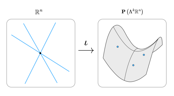
We have a Grassmannian variety [math]\displaystyle{ \mathrm{Gr} (k, n) }[/math] consisting of the k-dimensional subspaces of [math]\displaystyle{ \mathbb{R}^n }[/math]. The rational points on this variety can be identified with rank-k temperaments on a JI space with n primes.
Let [math]\displaystyle{ M }[/math] be an element of [math]\displaystyle{ \mathrm{Gr} (k, n) }[/math], spanned by basis vectors [math]\displaystyle{ m_1, \ldots, m_k }[/math]. We can embed the Grassmannian into a projective space using the Plücker map: $$ \begin{align} \iota: \mathrm{Gr} (k, n) & \to \mathbf{P}\left(\Lambda^{k} \mathbb{R}^n \right) \\ \operatorname {span} (m_1, \ldots, m_k) & \mapsto \left[ m_1 \wedge \ldots \wedge m_k \right] \, . \end{align} $$
Here, [math]\displaystyle{ \Lambda^{k} \mathbb{R}^n }[/math] is the k-th exterior power of our original space [math]\displaystyle{ \mathbb{R}^n }[/math]. The dimension of [math]\displaystyle{ \mathrm{Gr} (k, n) }[/math] is [math]\displaystyle{ k(n-k) }[/math], while the dimension of [math]\displaystyle{ \Lambda^{k} \mathbb{R}^n }[/math] is [math]\displaystyle{ \binom{n}{k} }[/math], which is typically much larger.
Examples
The space of lines through the origin is exactly projective space, so [math]\displaystyle{ \mathrm{Gr} (1, n) \cong \mathbf{P} (\mathbb{R}^n) }[/math]. In 3 dimensions, a plane through the origin is completely defined by its normal, so we get that [math]\displaystyle{ \mathrm{Gr} (2, 3) \cong \mathrm{Gr} (1, 3) \cong \mathbf{P} (\mathbb{R}^3) }[/math], the projective plane.
The simplest non-trivial case is [math]\displaystyle{ \mathrm{Gr} (2, 4) }[/math]. An element [math]\displaystyle{ M }[/math] spanned by two lines [math]\displaystyle{ x, y }[/math], can be represented as the matrix $$ \begin{equation} \begin{bmatrix} x_{1} & x_{2} & x_{3} & x_{4} \\ y_{1} & y_{2} & y_{3} & y_{4} \end{bmatrix} \, . \end{equation} $$
These are not 'proper' coordinates, as doing row operations on this matrix preserves the row-span. Put another way, we can always multiply by some [math]\displaystyle{ g \in GL_k (\mathbb{R}) }[/math].
The projective coordinates can be calculated by taking the determinants of all [math]\displaystyle{ 2 \times 2 }[/math] sub-matrices
$$ p_{ij} = \begin{vmatrix} x_i & x_j \\ y_i & y_j \end{vmatrix} \, , $$
which finally gives us
$$ \begin{equation} \iota (M) = \left[ x \wedge y \right] = \left[ p_{12} : p_{13} : p_{14} : p_{23} : p_{24} : p_{34} \right] \, . \end{equation} $$
Note the use of colons to signify that these coordinates are homogeneous.
Plücker relations
The coordinates must satisfy some algebraic relations called Plücker relations. Generally, the projective space is much 'larger' than the Grassmannian, and the image in the projective space is some quadric surface.
For the example above on [math]\displaystyle{ \mathrm{Gr} (2, 4) }[/math], the Plücker relation is
$$ p_{12} p_{34} - p_{13} p_{24} + p_{14} p_{23} = 0 \, . $$
Note that in this case, there is only one such relation, but in higher dimensions there will be many.
Rational points
A rational point [math]\displaystyle{ P }[/math] on [math]\displaystyle{ \mathrm{Gr}(k, n) }[/math] is a k-dimensional subspace such that [math]\displaystyle{ P \cap \mathbb{Z}^n }[/math] is a rank k sublattice of [math]\displaystyle{ \mathbb{Z}^n }[/math].
The same relations as above can be derived, where we represent P as integer matrix [math]\displaystyle{ M \in \mathbb{Z} ^ {k \times n} }[/math] and the projective coordinates similarly have entries in [math]\displaystyle{ \mathbb{Z} }[/math] instead. Because the Plücker coordinates are homogeneous, we can always put them in a 'canonical' form by dividing all entries by their GCD and ensuring the first element is non-negative.
Height
A height function is a way to measure the 'arithmetic complexity' of a rational point. For example, the rational numbers [math]\displaystyle{ \frac{3}{2} }[/math] and [math]\displaystyle{ \frac{3001}{2001} }[/math] are close to eachother, but intuitively the second is much more complicated.
We can define the height of a rational point simply as the Euclidean norm on its Plücker coordinates [math]\displaystyle{ X = \iota (P) }[/math]. $$ H(P) = \left\| X \right\| = \left\| p_1 \wedge \ldots \wedge p_n \right\| \\ $$
This is equivalent to the covolume of the lattice defined by P (also know as the lattice determinant), which can be easily computed using the Gram matrix. $$ \begin{align} \mathrm{G}_{ij} &= \left\langle p_i, p_j \right\rangle \\ \sqrt{\det(\mathrm{G})} &= \left\| p_1 \wedge \ldots \wedge p_n \right\| = \left\| X \right\| \, . \end{align} $$
In regular temperament theory, this height is usually known as simply the complexity.
Projective distance
Given a temperament, we want to have some notion of distance, so that we can measure how well the temperament approximates JI. Since we are talking about linear subspaces (which all intersect at the origin), the only thing that is sensible to measure is the angle between them.
In Euclidean space, one usually takes advantage of the dot product to measure angles. Given vectors [math]\displaystyle{ a, b \in \mathbb{R^n} }[/math], we famously have
$$ \frac{a \cdot b}{\left\| a \right\| \left\| b \right\| } = \cos (\theta) \, . $$
In projective space, there is an analogous formula, using the wedge product instead. Given some real point [math]\displaystyle{ j \in \mathbb{R^n} }[/math] with homogeneous coordinates [math]\displaystyle{ y }[/math], and a linear subspace [math]\displaystyle{ P \in \mathrm{Gr} (k, n) }[/math] with Plücker coordinates [math]\displaystyle{ X }[/math], we define the projective distance as
$$ d(P, j) = \frac{ \left\| X \wedge y \right\| }{\left\| X \right\| \left\| y \right\| } = \sin (\theta) \, . $$
Where we can take [math]\displaystyle{ j }[/math] to be the usual n-limit vector of log primes, so that [math]\displaystyle{ y = \left[ 1 : \log_2 (3) : \ldots : \log_2 (p_n) \right] }[/math]. Unlike the dot product formula, this works for subspaces of any dimension.
Since for any decent temperament this angle will be extremely small, we can take [math]\displaystyle{ \sin (\theta) \approx \theta }[/math].
