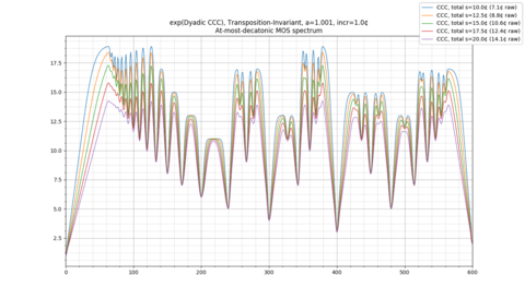
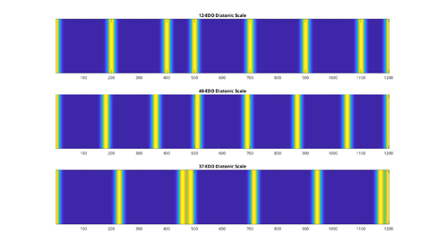
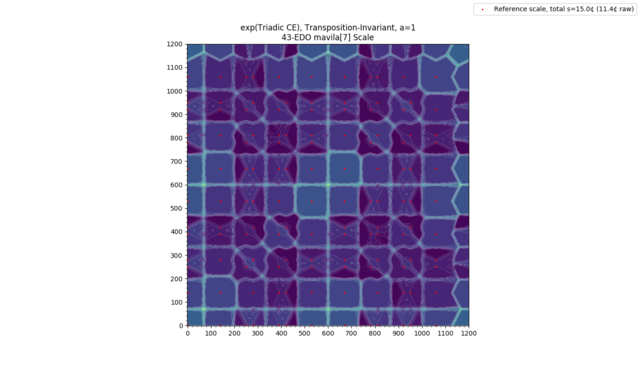
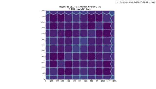
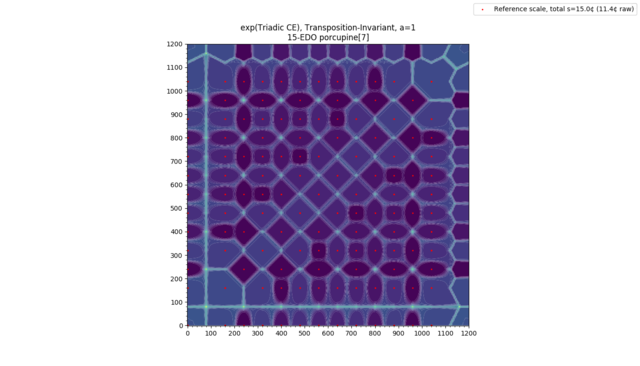
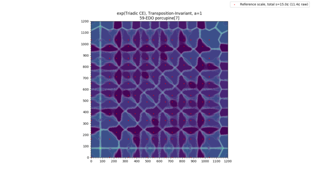
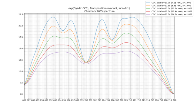
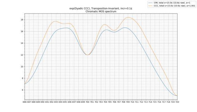
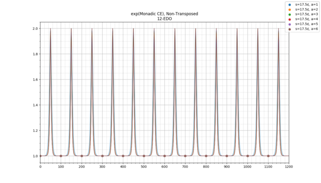
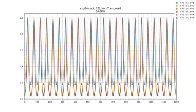
Categorical Entropy, Mutual Information, and Channel Capacity
The Categorical Entropy (CE), Categorical Mutual Information (CMI), and Categorical Channel Capacity (CCC) are simple additive white Gaussian noise (AWGN) models quantifying how distinct the notes and intervals in a scale are from one another. They were developed by Mike Battaglia and Keenan Pepper.
Introduction
One goal of xenharmonic music is to create music in new tuning systems that sounds "intuitive", "familiar", "intelligible", "hospitable", etc. To achieve this, some xenharmonic music theorists look for qualities exhibited by current or historical musical traditions (e.g. European/American, Middle Eastern, Indian, Indonesian musics), and attempt to generalize them. Such generalized properties may be used to determine families of tuning systems which share common features.
So far, much of this generalization has been focused on the search for tunings with chords that approximate simple fragments of the harmonic series, which produce psychoacoustic effects considered desirable in Western polyphonic music. To that extent, models have been developed such as Paul Erlich's "Harmonic Entropy," which attempts to quantify directly the "approximate harmonicity" of a chord, as well as the theory of regular temperament, which provides a method to find tuning systems that can approximate simple harmonic chords to within a desired accuracy level.
It has become clear, however, that there exist other phenomena than the harmonic ones described above that are similarly worth generalizing. In this article, we present a basic analysis of such phenomena that one might term "scalar" or "categorical."
Perception of Scale and Mode
Within a broad variety of musical traditions, many listeners exhibit some sense that there exists a background "scale" or "mode" that a piece of music can be "in" at some point in time, to which notes can either "belong" or not "belong." Listeners of these musical traditions typically learn to distinguish these scales from one another, either consciously or unconsciously, to the extent that they are usually able to determine which scale is the correct one to sing a melody in for some piece of music.
Virtually all of the world's musical traditions make use of scales in this way, to which they often ascribe different emotional qualities. Distinguishing between these scales, and more generally distinguishing between which notes are "appropriate" or "inappropriate" to play at a particular time in a piece of music, is usually considered important to most musical traditions. The general ability of most listeners to do this has been established in a large body of research by Carol Krumhansl and others.[1]
What is a "Note?"
The notion that scales are made up of discrete "notes" is less trivial than it would appear at first glance. For example, the tuning of each "note," in practice, can often vary considerably, even within a short time duration in a performance. Notably, techniques such as heavy vibrato are used deliberately in a wide assortment of musical traditions. Notes can also be adjusted intonationally to create various melodic or harmonic effects, or can be "bent" in a continuous glide.
We typically take for granted our ability to recognize, usually without much thought, such detunings as being "different tunings of the same note" rather than "two different notes." These phenomena routinely appear in music without disturbing the listener's sense of which note is being played, or where that note is located in the scale. And indeed, music would sound very different to us if our perception of notes, and all the melodic, harmonic, and "tonal" qualities they entail, were rendered totally unrecognizable every time a singer were 15 cents out of tune or used vibrato!
We consider the above an interesting feature of many musical traditions which we would like to model. However, some scales may lend themselves to being categorized into "background notes" more easily than others. We would like to understand how this works, quantify it, and find scales for which the perception of each note is as robust to mistuning as possible.
Categorical Perception and Ear Training
There is evidence in the literature that musical ear training enhances the ability of listeners to quantize the pitch spectrum into notes in this in the manner described above. This phenomenon that has been called "categorical perception" in the literature.[2][3] Listeners develop a heightened ability to perceive pitches as intonational variants of the underlying set of "categories" of notes. Each note develops a kind of "channel," "bandwidth," etc, surrounding the reference, and pitches within the channel tend to be perceived as representing an "intonational variation" of the reference category.
It has even been shown that trained listeners have an easier time distinguishing between equidistant intervals if they correspond to different categories.[4] For example, trained Western musicians typically have an easier time distinguishing between 325 and 375 cents than with 375 and 425 cents, since the former corresponds to a "minor third" vs a "major third", whereas the latter corresponds to two "major thirds." Listeners with AP typically an additional level of categorical perception for absolute pitches, rather than pitches relative to some tonic.[5]
One may be tempted, from the above literature, to conclude that years of ear training are necessary to be able to understand a new musical tuning. However, there is also research showing that listeners are good "musical tourists": they are generally able to identify, given a piece of music in a foreign musical tradition with which they have no experience, which notes are considered "appropriate" or "inappropriate" to play at a particular time in that piece.[6] This was studied explicitly in the context of North Indian and Gamelan music being played to Western listeners, and compared with expert "native" listeners: Western listeners were generally able to produce "rankings" of notes in "appropriateness" that were relatively consistent to those of the native listeners, although it is noteworthy that in expert listeners, the rankings were influenced somewhat by the note's perceived "membership" among a set of traditional scales.[7][8]
The above is evidence that, even absent any particular ear training regimen, the music has an intrinsic ability to "train" the listener's ear to develop some sense of the basic discrete "notes" currently being used, as well as their musical relevance through the course of a composition. Furthermore, given that many musical traditions can also exhibit vibrato, a range of intonational deviations, or in the case of Gamelan music, deliberate mistuning to create a chorus-like effect, it is reasonable to suggest that the listener's ability to do this exhibits some degree of robustness to intonational or tuning variations.
We consider that many of the world's musical traditions may have developed a structure that makes the music particularly "intelligible" on this level, both in the choice of scales that they use and in the way they choose to play them.
Categorical Perception vs JI "Interpretations"
Although this has not been studied explicitly in the literature, we consider there to be substantial evidence that this perception of different note "categories," or more generally interval or chord categories, does not necessarily correspond to the perception of different underlying JI "interpretations," or at least not in a simple one-to-one way.
A good example is traditional barbershop music. Barbershop quartets will switch between intonational variants of intervals to obtain the simplest JI representation possible - for example, a barbershop quartet may tune a "minor third" as 6/5 to bring it closer to 4:5:6, or as 7/6 if it is the top dyad of a dominant 7 chord, so as to tune the entire thing to 4:5:6:7. However, the intonational shift from 6/5 to 7/6 does not render it unrecognizable as an intonational variant of the original note, or disrupt the sense of scale position, in the same way it would if the intonation were shifted from 6/5 to 5/4. Were this not the case, barbershop music would sound very different.
That this is even possible is non-trivial, and tells us that these are two distinct phenomena. Indeed barbershop quartets get very good at this, to the extent that the entire barbershop tradition can be thought of as being a method of adjusting the JI interpretation of chords while preserving the scalar, melodic, and tonal structure of the music.
An Example: Categorical Experiments
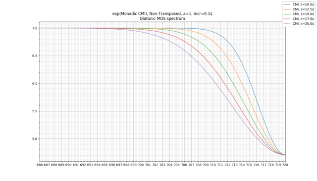
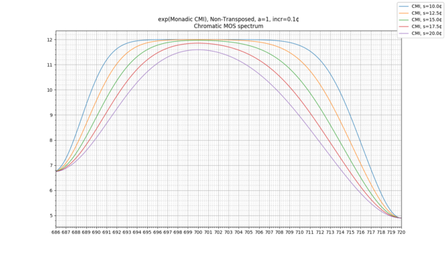
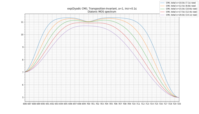
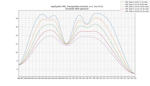
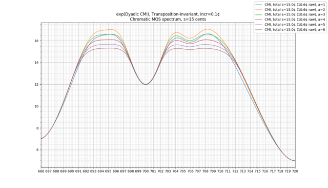
A good set of listening examples to demonstrate this are the "Categorical Experiments" by Mike Battaglia retuning the Bach Fugue in C major, where the fifth varies from 686 cents (7-EDO) to 720 cents (5-EDO).
When the fifth is tuned to a meantone tuning, such as 31-EDO, the thirds are decent approximations to 5/4 and 6/5. When the fifth is tuned to a superpyth tuning, such as 22-EDO, the thirds are now decent approximations to 9/7 and 7/6. However, many western listeners seem to agree that there exists some level of the music that remains intelligible through all of these retunings - the sense of scale, melody, and chord qualities such as "major and minor" - despite the differing JI interpretations used.
An easy way to see this is to compare the above to what happens if the fifth were tuned flat of 7-EDO, such as in mavila temperament. This doesn't just change the JI intonation of major and minor thirds, but actually causes them to switch places in the scale, so that the formerly "major" third is now ~300 cents, and the formerly "minor" third is now ~375 cents (as in 16-EDO). Examples of such retunings can be found in Mike Battaglia's Mavila Experiments for comparison. It is pretty easy to hear that formerly "major" pieces now sound "minor" and vice versa. Such a dramatic shift doesn't quite seem to happen when the 10:12:15's become 6:7:9's in the first set of examples, as happens when you move from 19-EDO to 22-EDO: while the intonational change is certainly noticeable, there is also some sense in which they retain the "minor" tonal identity, rather than changing to something entirely different.
Of course, further research is certainly needed, and the above should be considered as only representing anecdotal evidence from within the xenharmonic community. Furthermore, even within the community, there may be considerable variance in perception that should be studied and understood. However, there does seem to be some reasonable agreement that it is possible to retune the diatonic scale in a way that the JI interpretations change, but tonal identities such as "major" and "minor" do not, indicating that there is indeed another layer of information. For now, we consider this anecdotal evidence to be sufficient to proceed in exploring this principle further, which we will attempt to do with our model.
Developing New Categorical Perceptions: "Detwelvulating"
The above has led some listeners in the xenharmonic community to express the feeling that they may be unconsciously "categorizing" new tunings in the context of 12-EDO without realizing it. This sentiment goes all the way back to Ivor Darreg's message to "Detwelvulate!" One way to interpret this maxim is to get away from unconsciously interpreting the notes of new tunings as altered versions of 12-EDO categories, and rather develop a new categorical perception for the tuning at hand. This has led to questions about how this can be accomplished.
It is noteworthy that this is a relatively new way of thinking about this topic, and perhaps not the only way to accomplish this goal. For example, some composers have instead attempted to unlearn their 12-EDO based category system and not replace it with anything, freely exploring the use of the entire pitch continuum without any sense of discrete note or scale at all. Others have attempted to build a very large set of "universal categories," often JI-centric ones, in an attempt to cognize any scale by relating the notes in it to their categorized JI interpretations. These are certainly valid artistic approaches, and we would not wish to rule them out; however we will suggest a different path.
Our paradigm is to develop a different categorical perception for each individual tuning system, or at least for a sufficiently large chromatic scale from within that tuning system. These categorization schemes need not have anything to do with JI: for instance, 7/6 and 6/5 might be categorized as the same thing in one tuning (such as a "minor third"), whereas in another tuning, 8/7 and 7/6 might be categorized as the same thing, with 6/5 being mapped as an intonation of a different entity. The goal is to be able to wear different hats, so to speak, which are developed so as to be appropriate to each tuning, and switch between them when switching tunings.
We consider that many of the world's musical traditions may have developed a structure that makes the music particularly "easy to categorize" in this way. We will attempt to explore how this works in an information-theoretic model which is in some sense a "categorical" or "scalar" variation of Paul Erlich's Harmonic Entropy.
The Model: Scales as Musical "Information" Channels
We will use an information-theoretic model of a scale as a channel through which musical "information" of some type is represented and transmitted. The different scale notes and intervals are taken to "mean" different things with respect to the context of the music, which we will view as being representations of distinct messages of musical information.
Another way to phrase this is that this musical information is being encoded into the notes of the scale, transmitted when the scale is played, subjected to noise in the form of pitch or intonational deviations, and decoded when the listener deciphers the notes heard to obtain a mental construct of the original information transmitted.
The success of our model will hinge on our ability to quantify exactly how suitable a scale is for this purpose -- without making any assumptions at all about the nature of this "musical information." We will see that this is possible to do: we will simply assume information of the type we are describing exists, in some form, and that the perception of discrete scale steps or intervals serves as a signaling mechanism to transmit it on some meaningful level.
We will then ask: how easily can the scale notes and intervals be differentiated from one another, both for a "naive" and an "expert" listener? Whatever information these notes or intervals represent, we will not be able to correctly identify it if the intervals are so close in size that the listener cannot tell them apart.
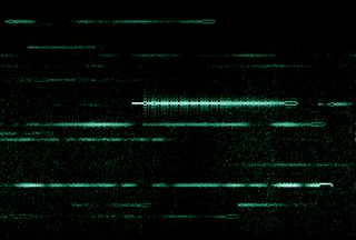
A good analogy is the picture to the right, representing multiple simultaneous radio transmissions taking place on multiple carrier frequencies. We know that information of some type is encoded into each carrier frequency, which "means" something to the listener when it is received and decoded. We don't know what the nature of this "meaning" is or what type of information is being transmitted. However, we do know that, if we would like any information to be transmitted at all, each carrier frequency must be given its own bandwidth, where it is adequately separated from other frequencies, in order to avoid interference.
Our model of a scale works in basically the same way: we do not know exactly what mysterious musical information is conveyed by the notes, or how the listener will interpret it, but we do know that we want the notes to be spread out enough to avoid interference from one another so that listeners can decipher them correctly.
Model Assumptions
In our model, we make two basic assumptions:
- Information of some nature is transmitted via the notes (or intervals) of a musical scale, such that some significant part of a listener's perception of music is determined by their perception of which note or scale position is being played.
- Different scale notes (or intervals) can generally be distinguished more easily from one another if they are further apart.
For the latter assumption, we assume that as a general rule, for example, listeners will be more easily able to distinguish between 300 and 400 cents than 330 and 360 cents, which are more likely to be confused with one another. As mentioned, this need not be 100% true in all circumstances, given the way that categorical perception skews subjective judgments about interval sizes, but we regardless consider this to be an unobjectionable general principle that is mostly true on average.
Using this principle, our aim is to quantify how "different" the intervals in a scale are from one another, which we view as an important perceptual quality of a musical scale. Our main thesis is that those scales for which each note is given as wide a "bandwidth" as possible will be easiest to categorize. This gives each note an allowance for real-world tuning variation, deliberate mistuning effects such as vibrato, or general "blurriness" in the auditory system of the listener, while still making it as clear as possible what notes are being played. Maximizing this "bandwidth" increases our chance that the note can be unambiguously interpreted without "interference" from competing ambiguous interpretations from nearby notes.
It is important to note that we don't necessarily place a musical value judgment on this property. Scales which have ambiguous intervals can also musically useful, as the ambiguities between intervals that are close but different can be used for musically expressive purposes. We simply would like to quantify, as a starting point, which scales have these kinds of ambiguous intervals in this way to begin with, and which don't.
The Nature of Musical "Information"
To gain a better understanding of what we are talking about, it is clear that there are many natural examples of the type of "musical information" described above, which are routinely transmitted and pertain to the perception of scale notes.
For example, different notes can transmit "modal" information relative to the listener's perception of which mode is currently being played. Notes can evoke a sensation of "fitting in" or "not fitting in" to the perceived modal context, either sounding modally "appropriate" or "chromatic." A sequence of notes that does not "fit in" could also be perceived as signaling a change to the listener's perception of which mode is currently being played, and hence constitute a different type of informational message: a "modulation."
On a different level, "melodic" information could additionally be transmitted that is purely cultural, in that a set of notes can resemble a musical phrase or "lick" commonly heard in a musical tradition. A sequence of notes could also convey some sense of melodic "contour," and cause the listener to form predictions about whether the next note will be higher or lower than the current one.
On yet another level, the information could be "tonal," in that intervals can represent Western tonal "functions" such as "minor third" or "perfect fifth," which we already know can be represented via a wide assortment of tunings. A note may evoke a sensation of being part of a particular chord from the Western tonal tradition. It may evoke the sensation of changing the sense of the "current chord," while preserving the general sense of scale and mode. Notes could be heard as arpeggiations of commonly played chords.
However, despite the seemingly endless possibilities for scales to convey information on different musical layers, we reiterate that it is not necessary to model any of this. Instead, our approach will enable us to simply model the capacity of the scale to serve as a discrete information channel for any type of information, assuming only that different scale notes communicate different informational messages. We will then model how distinguishable the individual scale notes and intervals are from one another at the reciever, even in the presence of tuning "noise."
Shannon's Theory of Information
Claude Shannon's theory of information was originally developed for use in telecommunications to serve this exact purpose: it enables us to speak meaningfully of the "information capacity" of a noisy channel without requiring us to know anything about what messages will be sent on it, or how they will be encoded.
An auditory example that makes the musical analogy particularly prominent is that of radio transmissions. In Ham Radio, the PSK31 format is a way to encode a message on a single carrier frequency. In a real-world radio spectrum, multiple PSK31 transmissions are always continuously beginning and ending at different times. If a sample of spectrum activity is simply played as an audio file, we hear different pitches slowly going in and out of existence, each representing a different message of some unknown nature. You can click on the right to hear an example of this; it sounds like various microtonal chords and scales slowly forming, modulating, and drifting. While we don't know what information the notes carry, we do know the carrier frequencies must be spaced far enough apart from one another to avoid interference. The PSK31 engineers needed to design their audio frequency-based transmission system to make the signal robust to noise without knowing literally anything at all about the nature of the "meaning" of the messages being encoded into the carrier frequencies. This is basically the situation that we face when designing a scale for "categorical clarity."
Imperatively, in both situations, we have the same limitation of not knowing anything about what particular information is being encoded. Indeed, it would be crazy if we were required to make guesses about the encoded semantic "meaning" of a particular radio transmission just to model how noisy the channel is! Likewise, we need not worry about this in our musical situation, only that whatever semantic "meaning" exists, it is somehow being represented by the pitches of the scale. The scale pitches are just another set of auditory frequencies that simply need enough breathing room to be robust from receiving errors in the presence of noise.
Shannon developed a set of techniques that enable us to clearly do everything listed above. We can measure how intelligible a signal is expected to be when sent on a noisy channel (the "Mutual Information"), and even maximize the amount of information that can be clearly sent across a noisy channel by changing the probability distribution of symbols being sent, so that "unambiguous symbols" are sent most frequently and "possibly ambiguous ones" less frequently (the "Channel Capacity"). We will use Shannon's theory to develop our metrics for a scale, which we call Categorical Entropy, Categorical Mutual Information, and Categorical Channel Capacity.
As we will see, we will obtain some noteworthy and basic results: for example, that mistuning a scale slightly can lead to an increase in clarity, by moving notes away from competing interpretations.
A Motivating Example: Diatonic Scale Perception Breakdown near 7-EDO and 5-EDO
To illustrate what we are talking about, consider the "Categorical Experiments", which demonstrate this effect for Western music and the diatonic scale.
While it is clear that some aspect of the general perception of note and scale is preserved even under a wide variety of deformations, it can be seen that this perception begins to break down near the extremes of 7-EDO (with L/s = 1/1) and 5-EDO (with L/s = 1/0).
When the fifth approaches that of 7-EDO, the chromatic semitone approaches 0 cents, so the "minor," "major," "augmented," and "diminished" versions of each interval begin to converge in size and become ambiguous with one another, and it becomes more likely that the listener confuses major and minor third and so on. As we get to 7-EDO, these intervals become identical, and at that point, the scale may start to shift into a totally different perception entirely.
Likewise, when the fifth approaches that of 5-EDO, the diatonic semitone approaches 0 cents, so that the "major second" and "minor third" converge in size and become ambiguous, as do the "major third" and "perfect fourth," the "perfect fourth" and "diminished fifth," and so on. For instance, if the fifth is tuned to 714 cents as in 37-EDO, within the context of the diatonic scale, a Western listener may perceive the 454 cent interval as representing a common practice "major third," and the 486 cent interval as representing a common practice "perfect fourth." However, these intervals are close enough that the listener may occasionally think that the 454 cent interval is the 486 cent interval and vice versa, and hence interpret the current interval as a representation of the "perfect fourth" rather than the intended "major third."
It is noteworthy that the same "breakdown" occurs to a much smaller extent as the tuning converges on 12-EDO, the tuning where the diatonic scale's L/s = 2/1. In this situation, the diminished fifth and augmented fourth converge in size and become ambiguous. Likewise, in the context of the harmonic scale, the augmented second and minor third become ambiguous, as do the major third and diminished fourth. However, in each of these cases, the "total level of ambiguity" is in some sense much less than in 5-EDO or 7-EDO, where every single interval in the diatonic scale has become ambiguous. We will want a model that scores this appropriately. (As we will see, other MOS's sometimes fare much worse than the diatonic scale when tuned to the L/s = 2/1 point.)
Confounding Factors: Variance in Hearing, Musical Training, Joint Distributions
We note that whether 37-EDO is ambiguous enough to produce the effect described above is likely variable from person to person. Some listeners may be still capable of distinguishing between the major third and perfect fourth in this situation without much trouble. For those listeners, moving to the generator of 43\72, or 717 cents, may cause more trouble, as the "major third" is now represented by 467 cents and the "perfect fourth" is now represented by 483 cents. For other listeners, 37-EDO may already be at the point where the diatonic semitones are too small to distinguish, so that their ears "give up" and they hear the entire thing as a pentatonic scale with some intonational variations. Those listeners may not have the same perception in 32-EDO or 27-EDO, where the diatonic semitones are larger.
Lastly, we note that musical training may alter the perception of the above significantly, and perhaps serve as a possible confounding effect. For example, expert listeners may be able to use musical context to gain additional "clues" as to which scale interval is being played, even in the case of extreme tuning ambiguity. This may hold even to an extreme degree that even in 5-EDO or 7-EDO, people can still sometimes perceive instances of "major" and "minor thirds" occurring even if they are tuned identically, based on learned patterns from musical context. This is similar to how listeners can perceive a difference between "augmented seconds" and "minor thirds" in Western music, even though these intervals are tuned identically in 12-EDO (and most listeners have had little to no prior exposure to different tunings of the diatonic scale).
In these situations, for such listeners, the "breakdown point" does not lead to a total breakdown in scale perception. However, we still consider that as a general rule, it is certainly easier to distinguish different intervals on average when they're tuned further apart from one another. Hence, we consider this distinctness criterion to be worth maximizing, particularly since in xenharmonic music we are often concerned with exploring tunings for which we have no prior musical setting to draw from.
Regardless of where the "breakdown point" may be for a particular listener, it is clear that at some point on the way to 5-EDO, ambiguities of the type mentioned will begin to arise and become frequent. Our model will represent this variability with a single free parameter called [math]s[/math] that represents the "fineness" of hearing, similarly to Paul Erlich's Harmonic Entropy model. The listener will be able to adjust [math]s[/math] to see how robust a scale is to these types of mis-decodings.
Lastly, we also note that we are only modeling the individual notes of a scale, whereas in real musical situations, the surrounding notes (in a melody or chord) further give the listener information about what notes are being played. That is, the set of sequences of notes are nontrivially jointly distributed, so that the listener is more easily able to determine what notes are being played given a fragment of the surrounding context than if they are played in isolation. An interval which is "ambiguous" when played in isolation may quickly become unambiguous once the listener hears the following notes and is able to identify the scale being played; this ability will clearly vary with musical training. It would be interesting to extend the model to handle these kinds of situations, but we will leave that for future research.
Within the Model
In our model, what is happening is that in these situations is that the listener can simply become confused about which interval scale step they are hearing, because the intervals involved do not have enough "bandwidth" to be free from interference from other intervals. This can lead to an incorrect interpretation of the musical information the notes are supposed to represent.
There is a very important caveat here. When we say that the listener may start to confuse major and minor thirds, whole and half steps, etc, as things get closer to 7-EDO, we have made a very important assumption: that the *goal* of the music is to have these things be different to begin with in such a way that is musically meaningful (as in Western music). Or, to be precise, we are assuming that some reference scale - the diatonic, for instance - has within it a set of intervals which are important to be able to tell apart from one another, and that we would like to measure how well some tuning of this scale lets listeners do that. But we note that there is clearly some point at which two closely-tuned intervals switch from sounding two different "types" of interval, albeit ambiguously tuned, to sounding like they are simply intended to be one "type" of interval to begin with.
This phenomenon is most familiar in Western music with 12-tone circulating temperaments such as Werckmeister III: there are many different sizes of fifth, for instance, but they all sound like slight variations on the same archetypical interval of the perfect fifth. This ought to be thought of as a feature, not a bug: if one's goal is to design a 12-tone well temperament, it would make no sense to evaluate the slightly different fifths negatively as being "ambiguous and difficult to tell apart." Rather, one would certainly *want* the fifths to be close enough in size that they all sound like different variations of the same thing. That's the entire point!
Of course, our goal here is not just to measure how good different tunings of scale are at representing Western tonal functions. The real question is: as the diatonic scale is tuned closer and closer to 7-EDO, at what point does it stop sounding like an ambiguous diatonic scale, and start sounding like something else - perhaps a slightly unequal "well temperament" of 7-EDO?
We will not attempt to answer these questions in any absolute sense, but rather present our analysis as follows: given some scale, we will present metrics that simply quantify how clearly the intervals in the scale can be differentiated from one another, by measuring how many "effective" types of easily-differentiable-interval are present in the scale (the "alphabet size" of the scale). The higher this quantity is, the more "information" the model claims the scale is capable of transmitting unambiguously. If two intervals are very unambiguous and different in size, the metric will count them as two "effective" types of interval. As they get closer and closer, the metric gracefully starts to count them instead as one effective type of interval in a smooth way. (Again, of course, it is up to ones musical judgment if this is a good thing or not.)
The main idea is that using these metrics, we can ask questions like:
- Given some archetypical reference scale, how categorically "stable" is the perception of that scale relative to itself?
As we will see, the model predicts that there are many scales with the interesting property that, even if they are treated as some kind of idealized reference scale, are not their own "optimal" tuning with respect to this quantity. That is, the model will suggest adjustments in tuning which make different intervals easier to differentiate from one another.
Some Last Caveats
Of course, this is not the only quantity that matters, so it should be used alongside other useful metrics. For instance, naive application of this model will naturally suggest that the "ideal" scale is something like a Golomb ruler, where every single pair of notes is some unique interval size. While this technically satisfies the criteria of maximizing this one particular quantity, this is perhaps not ideal for other musical reasons, where we may be most interested in scales with a max-variety of 2 or 3. So, of course, we expect that composers will tend to incorporate these additional criteria as they see fit, perhaps using the model only on MOS scales to see which ones maximize this quantity.
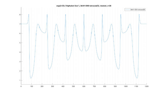
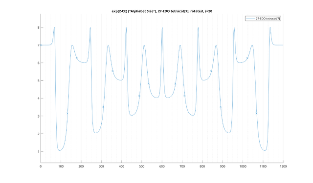
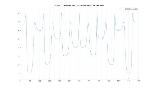
Another caveat is that many MOS's from "good" regular temperaments tend to form rather ambiguous, quasi-equal MOS's that don't fare well on this sort of metric (such as tetracot[7]). Given such a scale, this model, one way or another, will basically suggest making it less quasi-equal - somewhat closer to the tuning of "tetracot[7]" in 13-EDO. And indeed, if categorical clarity is all that we care about, it is certainly much easier to tell the intervals of the 6L1s MOS apart in 13-EDO than in 34-EDO - but this improvement has come at the cost of the approximation to just intonation. So we leave it up to the composer how they'd want to make that tradeoff.
In short, we really wanted to just focus on the categorical analysis of scales with this particular model, leaving to future research the best way to combine with other models focusing on other things (such as Harmonic Entropy).
Formal Model Definition: Probabilistic Scales
NOTE: this part gets fairly technical, so you may want to just skip below to the example pictures. And then look at the examples for CMI and examples for CCC!
We will begin our model by extending the usual definition of a scale to include probabilistic pitch deviations.
That is, rather than each scale degree having a single, unambiguous, deterministic tuning, the tuning will instead be given a random variable, representing a probability distribution of possible realizations. The mean of this random variable will be given by the scale degree's reference pitch.
We will then place a probability distribution on the scale degrees themselves. That is, we will consider certain scale degrees to have a larger probability of being played than others. Intuitively, we would like the most probable note to be considered as the "tonic," the second-most probable to be considered something like a "reciting tone," etc. If we would like a scale which does not have any such prioritization of intervals, we will represent it by a scale which has an equal probability for all scale degrees (i.e. a uniform distribution).
These two probability distributions will enable us to use the techniques of information theory to evaluate various "categorical" properties of the scale. In particular, it will enable us to view the scale as a probabilistic information channel with an associated mutual information representing how "noisy" it is.
Before we define this, however, we will need to clarify which version of the word "scale" we are talking about.
Preliminaries: What is a Scale?
Although the term "scale" has been used in different ways, we will use a notion of scale that is
- invariant to the choice of any particular tonic or "mode"
- invariant to the choice of any particular transposition or "key"
For example, in 12-EDO, we want to consider C major, D dorian, E phrygian, etc, as well as C# major, D major, etc, all as being different modes and transpositions of the same basic scale: the diatonic scale.
In this text, to keep things simple, we will generally assume that we are working with octave-periodic scales. However, it is fairly trivial to change everything to have a different interval of equivalence, such as in the Bohlen-Pierce scale, or even to use non-periodic scales such as Maqam Saba, if so desired.
When we work with octave-periodic scales, we will generally represent the scale as a single octave, for which each note is assumed to represent all octave-transposed versions.
Lastly, we will define the notes of our scale by specifying them in cents, relative to some arbitrary pitch in the scale we choose as having the special value of "0 cents." Note that this choice of pitch does not signify a choice of tonic, or "most important" note - rather, that type of information is more adequately represented by the probability distribution on each notes, so that the most probable note can be considered the tonic. However, we generally need to pick some note to be the 0 cent reference, so that there is more than one way to represent the same scale: for example, the sets {0, 200, 400, 500, 700, 900, 1100} (12-EDO Ionian) and {0, 100, 300, 500, 600, 800, 1000} (12-EDO Locrian) are considered to both be equally valid representations of the same diatonic scale.
Making Scales Probabilistic
We will first begin by placing the exact tuning of the notes in a scale into a probabilistic superposition. That is, the exact tuning of each note will be given by a probabilistic point-spread function.
As example, let's look at the 12-EDO octave-periodic diatonic scale, where the major mode is chosen as a reference point. We will start with a usual scale as a set of exact musical pitches:
$$ S = \left\{ 0, 200, 400, 500, 700, 900, 1100 \right\} $$
We will first replace the above tunings with a probabilistic tuning, where the mean is centered on each scale degree. Let us notate that as follows:
$$ S = \left\{ \overline{\mathbf{0}}, \overline{\mathbf{200}}, \overline{\mathbf{400}}, \overline{\mathbf{500}}, \overline{\mathbf{700}}, \overline{\mathbf{900}}, \overline{\mathbf{1100}} \right\} $$
where the bold and overline means we are defining each entry to be a random variable that is "approximately" the value given (e.g. takes it as a mean), but with some nonzero variance in the tuning (and possibly other nonzero moments as well).
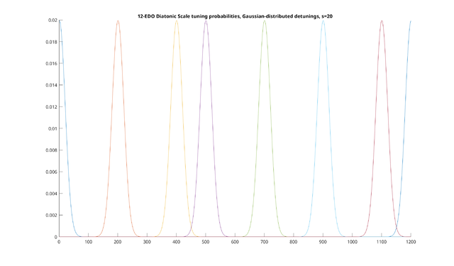
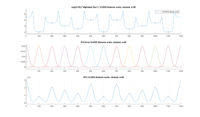
A typical choice for the random variable would be to make each note Gaussian-distributed, wrapping at the octave, with some standard deviation s. If we do so, and we set s=20 cents, we get the following probability distributions for each note:
This means that for each reference note, we should expect the tuning of the note to be distributed according to the curve in question. Increasing the value of s widens the curves, so that detunings are more common, whereas decreasing narrows them. (Note the value of 20 cents here may be slightly too wide for the diatonic scale, but it's a decent starting point, and is useful just to show the basic principle.)
Note that this probabilistic spreading of pitch can be viewed as representing the sum total of a wide range of sources of tuning deviations: deliberate performance bends, unintentional tuning deviations, vibrato, or even perceptual pitch "blurring" effects introduced by the auditory system. It is not necessary that each reference note have the exact same probability distribution of possible tunings, or even that the notes be Gaussian distributed, but for now we will assume identical Gaussian distributions on each note. It is then assumed that the ability to adjust the "s" parameter will give sufficient flexibility to represent the total degree of tuning deviation, on average.
Lastly, we will not only use scales where the notes have probabilistic tunings, but where the notes have probabilities of being played to begin with. For example, if we want to represent the major mode, we might use something like the following probability distribution:
$$ S = \left\{ \begin{align} \overline{\mathbf{0}}:& 21\%, \\ \overline{\mathbf{200}}:& 11\%, \\ \overline{\mathbf{400}}:& 15\%, \\ \overline{\mathbf{500}}:& 14\%, \\ \overline{\mathbf{700}}:& 17\%, \\ \overline{\mathbf{900}}:& 12\%, \\ \overline{\mathbf{1100}}:& 10\% \end{align} \right\} $$
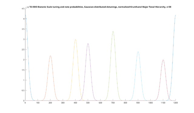
These probabilities were created from Krumhansl and Kessler's major tonal hierarchy, by taking the relative ratings of each note in the major scale and normalizing the sum to 100%. Note that the original hierarchy does not give explicit probabilities or "strengths" for each note, just simply a relative ranking on notes, so this is intended to simply be an informal analogue just to illustrate the basic idea. If we use the above probability distribution on notes being played, and combine it with the probability distribution on tunings from above, we get the following set of probability distributions:
The important thing to note is that, as can be seen in the above picture, these probability distributions can sometimes overlap. That is, given the tuning "450 cents," there is some probability that it is a detuned version of the "400 cent" reference note, played sharp, or a detuned version of the "500" cent reference note, played flat. Indeed, there is technically a nonzero probability that it is even an extremely detuned version of the 1100 cent note, played 650 cents flat, although the probability is so small that it is basically zero.
As we will see above, this is the basic feature on which the entire model rests: that multiple notes can be detuned to generate the same realization. We can then ask where and how often these "clashes" occur, and obtain a bunch of information-theoretic metrics modeling various aspects of our scale.
To delve further, we will need to simplify our notation somewhat.
A Better Notation
Above, we formalized our scale [math]S[/math] as a "random variable of random variables". That is, first there is a random variable determining which note is played, and then for each note, a second random variable determining what the tuning of that note is. It so happens that it is much easier to represent this mathematically if, rather than thinking of this as a single random variable [math]S[/math], we think of it as two jointly-distributed random variables:
- [math]X[/math], a discrete random variable representing "reference notes" in a "reference scale," with an associated probability of each reference note being played
- [math]Y[/math], a continuous random variable representing the "output" tuning that ends up being played, one way or another, superimposed for all possible choices of [math]X[/math]
In other words, we want [math]X[/math] to represent the discrete steps of our scale. We can name the outcomes of [math]X[/math] anything we want: relative names like "P1", "M2", "M3", etc, or absolute names like "C", "D", "E", etc or anything else. [math]X[/math] is a probabilistic superposition of these reference notes, weighted by the probability of each one being played. In the absence of any particular probability distribution for [math]X[/math], the uniform distribution with all notes having equal probability can be thought of as the best "default" distribution.
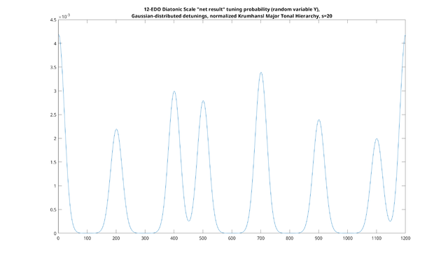
[math]Y[/math], on the other hand, represents the probability of each exact tuning in cents somehow being generated, one way or another, from the different values of [math]X[/math]. This can be thought of as the sum of the probabilistic tuning curves for each note in [math]X[/math], weighted by the probability of that note. To more easily visualize [math]Y[/math], here is a plot of the probability of [math]Y[/math] of the major scale from above, weighted by the normalized Krumhansl's major tonal hierarchy:
This is just the sum of all the Gaussian curves from the last picture. As you might expect, there are local maxima of probability for each note in [math]X[/math]. Also, as you can see, in this scale, there is a slightly higher probability of 450 cents being generated than 300 cents: 300 cents is not in the scale at all, and would need to be bent ~100 cents from either of its nearest neighbors, whereas 450 cents can be generated by a ~50 cent bend from either of its nearest neighbors. (Of course, this is a simplification due to the identical Gaussian mistunings and the lack of any "chromatic" notes in our scale; adding chromatic notes to the scale with a small probability would likely change this result.)
Given the above formalism, we can then talk in the usual manner of the following probabilities:
- [math]P(X=x)[/math] - the probability of the reference note [math]x[/math] being played from [math]X[/math] to begin with, apart from tuning
- [math]P(Y=y)[/math] - the probability of the output tuning [math]y[/math] in cents being generated somehow from all possible [math]X[/math]'s, one way or another
- [math]P(Y=y|X=x)[/math] - the conditional probability, given that the reference note played is [math]x[/math], that the output tuning is [math]y[/math] cents
- [math]P(X=x|Y=y)[/math] - the conditional probability, given that output tuning was [math]y[/math] cents, that [math]x[/math] was the reference note that generated it
So in our current example:
- [math]P(X=x)[/math] is the probability distribution on reference notes, which is the "major tonal hierarchy" probability distribution we derived above by normalizing Krumhansl and Kessler's result
- [math]P(Y=y)[/math] is the last curve shown above, the probability distribution on output tunings being generated "at the end of the day"
- [math]P(Y=y|X=x)[/math], given some chosen reference note [math]x[/math], is simply the aforementioned Gaussian curve representing the probability distribution of tunings for [math]x[/math].
- [math]P(X=x|Y=y)[/math] has not been previously talked about, but is very important: given a particular realized tuning such as "450 cents", this is the probability, for each [math]x[/math] that it was a generated as a "detuned version of" that [math]x[/math].
The third one is particularly important. For example, if we give our "400" cent reference interval the name "M3", then [math]P(Y=y|\text{M3})[/math] is the Gaussian probability distribution corresponding to the thing we previously called [math]\overline{\mathbf{400}}[/math].
The fourth one will be seen, later on, to form the basis of our notion of Categorical Entropy.
Example Outcomes
Given that we now have our two-variable formalism, we can talk about particular outcomes of our scale. An outcome, in this case, will be a particular note and a particular tuning, or formally, a particular outcome from [math]X[/math] and a particular outcome from [math]Y[/math], which we will write using the notation Interval name: tuning. If we name the notes of our scale "P1", "M2", "M3", etc, then here are some example outcomes:
$$ \text{M2}: 200¢ \\ \text{M2}: 190¢ \\ \text{M2}: 210¢ \\ \text{M3}: 400¢ \\ \text{M3}: 386¢ \\ \text{P4}: 504¢ \\ \text{M3}: 450¢ \\ \text{P4}: 450¢ \\ \text{P4}: 1199¢ $$
The first three are outcomes where the major second was chosen to be played, and tuned three different ways. Next is a major third tuned exactly to the reference at 400 cents, and a major third detuned slightly to 386 cents (close to 5/4). Next is a perfect fourth, tuned 4 cents sharp of the reference. These are all fairly straightforward.
Next we have our two most important examples: a major third tuned very sharp, to 450 cents - (relatively uncommon, but possible), and a perfect fourth tuned very flat, also to 450 cents (likewise, uncommon, but possible). The main thing to note here is that for our probabilistic scale, these are two distinct outcomes. That is, the outcome here isn't just the realized tuning of "450 cents": it is the combination of the 450 cent tuning, and the intended reference note which has been tuned that way.
In other words, an outcome of our probabilistic scale should be thought of as representing "the whole truth": the intended reference note in the mind of the performer, and the realized tuning that is then played. Both pieces of state are represented.
Lastly, we have a perfect fourth tuned to 1199 cents - a deliberately bizarre example, just to show you that this is technically a possible outcome, even though the chances of it happening are so low that you may as well think of it as zero!
Probabilistic Scales as Information Channels
A very useful way to look at the above is where [math]X[/math] is an "input," perhaps a note on a piece of sheet music, that is being sent into some abstract system: the performer's instrument, interpretive choices, and the auditory system of the listener, which ultimately outputs [math]Y[/math] as a result. As a result, the pair [math](X, Y)[/math] can be thought of as representing a channel, one of our previously-described goals.
In a typical musical situation, a listener does not have direct access to the original input [math]X[/math], the original reference note the performer was intending to play. Rather, the listener only has access to their perception of the realized tuning [math]Y[/math] - the received "output" of the channel - and must infer the value of [math]X[/math] based on that. Note that this need not be a conscious process, as in naming the interval an ear training test, but for most listeners may be a largely subconscious one simply involving a general perception of whether the heard note fits into the current scale or not, or an understanding of how to correctly sing along with a melody.
For many possible received values of [math]Y[/math], the tuning will be close enough to some reference in [math]X[/math] that it can be unambiguously decoded. A "good" scale will be one which is relatively easy to decode in this way, where the most commonly heard "outputs" yield only one realistic guess of what the "input" most likely was.
The basic challenge with such inference is when a value of [math]Y[/math] is received that could have been generated with roughly equal probability by multiple values of [math]X[/math], such as our 450 cent example. In that situation, we now have multiple competing interpretations for our interval, for which the listener shall have to struggle to use additional sources of information to guess what [math]X[/math] is. We would like our scales to have these situations happen relatively infrequently. In our example, the ambiguity of 450 cents doesn't pose much of a problem because we don't expect it to be played very often, since it's a rather extreme deviation from the nearest reference. However, as we will see later, it is possible for scales to yield ambiguous tunings much more frequently, even scales which are considered "good" by other criteria.
Limitations and Future Extensions of this Model
In real music, there are many factors that can influence the musical interpretation of an "ambiguous" note or interval - the [math]X[/math] that is inferred from some given [math]Y[/math] - such as: the musical context and surrounding notes, the harmonic context of additional notes being played, fragments of melodies that listeners recognize, and so on.
In order to get to "the next level" of musical realism in our model, we have to extend our probabilistic scale - we can look at sets of notes played simultaneously (e.g. chords), or sequences notes (e.g. melodies), or sequences of sets of notes (e.g. chord progressions) - which will have a highly interesting and non-trivial joint distribution, which may differ from musical style to musical style, something which we will do in future research. Then, when an ambiguous note is played, we can also include a fragment of musical context from the surrounding notes/chords/etc, which may alter the relative probabilities of the note being inferred (rather than the note being played in isolation).
In some sense, we would like to model how good a scale *could be*, given an entire culture that uses it, with expert musicians and listeners for that scale, and an entire body of music that people know, etc. Our model is clearly just a starting point that falls short of a goal as extreme as *that* - but we will see later that, even within just the simple model, there are some basic metrics we can look at to begin to head into this direction. One example is the Categorical Channel Capacity, in which we look at the *best* possible distribution on the notes of a scale, in which unambiguous notes are played "just enough" to add some spice, and ambiguous notes are played more frequently. An extension of these things to an expanded probability distribution of multiple note sequences, chords, etc would be quite radical and enlightening in revealing the "best way" to use a scale; it would be quite interesting to see if real-world musical traditions tend to follow any of the results such metrics would give.
For now, our model of a probabilistic scale is as basic as possible - it simply looks at a scale and a probability distribution on that scale. This can be thought of as a very basic "average" on all possible melodies, chords etc, of how much each note or pitch class "matters" and how "probable," "salient," "relevant," or "generally likely to be played" it is. Our goal is simply to get as much mileage from this simple starting point as possible, with any results being understood to be kind of a basic guideline or starting point from which things may somewhat vary in different real-world musical situations.
We also want to emphasize that, although we are quantifying some kind of "ambiguity" that a musical scale an have, we do not necessarily place any musical value judgment on scales either having or not having this property. Rather, our view is that this property simply "exists," and we want to quantify it. Intervallic or pitch ambiguity can be very musically useful, particularly in the hands of an expert musician who is able to use it expressively to play with the audience's expectations. Clearly, the "threshold of ambiguity" will be much higher if the scale is being played by an expert musician, and using real melodic phrases that are recognized by expert listeners - and we hope that the [math]s[/math] parameter in the model provides some way to adequately model some of this variance. And lastly, we note that, even for "expert" listeners, there will always be some scales, such as those having many steps that are only 1 cents wide, for which it will be very difficult for the notes in the scale to sound different from one another at all. But of course, there are many musically interesting things you can do with scales that have such extreme "microtones," even if the intervals [math]400¢[/math] and [math]401¢[/math] are not quite as inherently "categorizably different" as [math]400¢[/math] and [math]300¢[/math] are.
Now that we have formalized all this, we have everything we need to create our model of Categorical Entropy.
Categorical Entropy
Given the above, the most basic quantity relevant in inferring a reference note from a realization is the conditional probability
$$ P(X=x|Y=y) $$
or the probability, given some received output [math]y[/math], of each [math]x[/math] being the thing that generated it.
This is automatically determined as a derived quantity once the probabilities [math]P(X=x)[/math] and the spreading functions [math]P(Y=y|X=x)[/math] are set. Given those two things, we can then use Bayes' Theorem to get:
$$ P(X=x|Y=y) = P(Y=y|X=x)\frac{P(X=x)}{P(Y=y)} $$
Our goal, then, is to determine how much, for each tuning realization [math]y[/math], the above probability distribution on values of [math]X[/math] tends to focus on only one choice. If the above distribution yields a 99% chance of being one particular value of [math]X[/math] and 1% on the rest combined, it is relatively unambiguous. If it yields a 49% chance on one, a 49% on another, and a 2% chance on the rest, it is more ambiguous.
The traditional way to measure this is Claude Shannon's definition of the entropy, which for this particular random variable is defined as follows:
$$ H(X|Y=y) = -\sum_{x\in X} P(X=x|Y=y) \log P(X=x|Y=y) $$
This is the Raw Monadic Categorical Entropy (1-CE) of the note [math]y[/math] with respect to the scale [math]X[/math]. Typically, the base of the logarithm is chosen to be either [math]2[/math] or [math]e[/math], representing either "bits" or "nats"; we will leave it open here.
Higher values denote that the interval is more ambiguous, whereas lower values denote that it is less ambiguous.
The terms "raw" and "monadic" will be made clear shortly. As we will see, a "transpositionally-invariant" notion of CE is much more useful, but defining the raw entropy in this way is a good starting point.
Raw Monadic Categorical Entropy (1-CE)
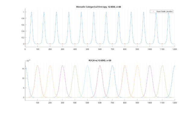
Let's look at the 1-CE for the 12-EDO scale, with all probabilities equal at 1/12, setting [math]s[/math] to 20 cents. If we do so, we get:
The curve above is the entropy; the red "X"'s are the exact scale degrees (meaning the reference notes of 12-EDO). We can see that, as expected, intervals that are close to the reference are low in entropy, whereas intervals that are far are high in entropy.
The lower curve shows the point spread function for each interval in the 12-EDO reference. We note that these curves bear some resemblance to the "identification functions" in Figure 1 of Siegel 1977, as well as Figure 1 of Burns 1978. (We will not present a plot of the point spread functions again, since they're fairly simple to understand.)
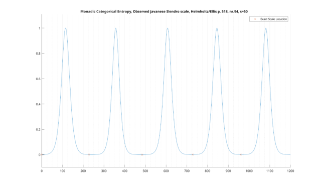
We can do the same for the notes of Slendro - we will use Helmholtz/Ellis's reference (p. 518, nr. 94, "slendro.scl"), set to 0, 228, 484, 728, and 960 cents, wrapping at the octave. As our intervals are much further apart, we may as well increase the value of [math]s[/math] to 50 cents, to demonstrate the difference. Doing so, we obtain
We can see we have gotten a similar result. Interestingly, you will note that the exact scale degrees (given by the red "X"'s in the above plot) are not exactly located at the minima of entropy - something that will become very important later.
Raw Dyadic Categorical Entropy (2-CE)
We can also increase the number of notes in our model. Rather than simply comparing a note to the reference, we can compare pairs of notes to pairs of notes in the reference to obtain the Dyadic Categorical Entropy (2-CE).
To do so, we will assume each note in the dyad can be independently mistuned from its reference by the same amount, given again by the parameter s.
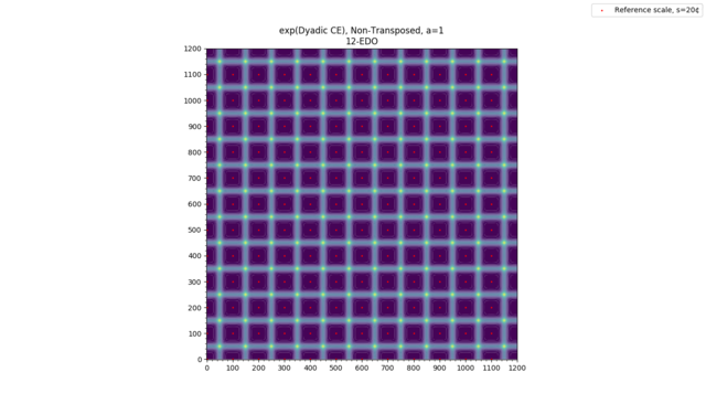
Here is an example of our dyadic 12-EDO from before, with all notes at equal probability:
So far, this is fairly simple: for 12-EDO as a reference, the lowest 2-CE triads will be found when tuned exactly to 12-EDO, and increase in 2-CE as they are detuned. We will see that things will get more interesting for different scales.
Raw n-adic Categorical Entropy (n-CE)
Before we can move to non-equal temperaments, we want to note that we can extend the above principle to get a notion of 3-CE, 4-CE, etc, although we will not be able to plot this here.
In general, we can do so by changing our random variables [math]X[/math] and [math]Y[/math] as follows:
- [math]X_n[/math], a discrete random variable of "reference chords", and an associated probability of each reference chord being played
- [math]Y_n[/math], a continuous random variable representing the possible "output" chord tunings that can be generated somehow from all possible reference chords in [math]X_n[/math], with an associated probability of each tuning being generated one way or another. This can be viewed as a tuple of cents, representing the tuning of each note relative to the "0 cent" reference.
Given that, we can again look at our basic probabilistic quantities as follows:
- [math]P(X_n=x_n)[/math] - the probability of the n-note reference chord [math]n_x[/math] being played to begin with
- [math]P(Y_n=y_n)[/math] - the probability of the tuning of the n-note output chord [math]y_n[/math] being generated somehow from all possible reference chords
- [math]P(Y_n=y_n|X_n=x_n)[/math] - the conditional probability, given that the reference chord being intended is [math]x_n[/math], that the output tuning is [math]y_n[/math]
- [math]P(X_n=x_n|Y_n=y_n)[/math] - the conditional probability, given that the output chord was [math]y_n[/math], that [math]x_n[/math] was the reference chord that generated it
The quantity [math]P(Y_n=y_n|X_n=x_n)[/math] represents the tuning probability distribution for each reference chord [math]x_n[/math]. Generally, we will want each note in the n-chord to be able to be independently mistuned by the same distribution we used in the monadic case. So for example, if our original tuning distribution was a Gaussian distribution, this would be a "white" multivariate Gaussian distribution with the same value of [math]s[/math] on each note (so the covariance matrix would be a diagonal matrix of all [math]s^2[/math] entries).
Given the above, the n-adic Categorical Entropy is defined as:
$$ H(X_n|Y_n=y_n) = -\sum_{x_n\in X_n} P(X_n=x_n|Y_n=y_n) \log P(X_n=x_n|Y_n=y_n) $$
Generally, we will want our list of "reference chords" to be those taken from some scale, i.e. for n-adic CE, we the set of all n-ads contained in a scale. In set-theoretic terms, this is called the n'th Cartesian power of the scale, containing all n-tuples of notes in the scale (including duplicates, and with different orderings counting as different notes).
For example, for the 12-EDO pentatonic scale (notated as C-D-E-G-A), to get 2-CE, the 2nd Cartesian power would be the following:
(C, C) (C, D) (C, E) (C, G) (C, A)
(D, C) (D, D) (D, E) (D, G) (D, A)
(E, C) (E, D) (E, E) (E, G) (E, A)
(G, C) (G, D) (G, E) (G, G) (G, A)
(A, C) (A, D) (A, E) (A, G) (A, A)
This would be the sample space for [math]X_2[/math], assuming that [math]X[/math] is the pentatonic scale. You can see that both (C, G) and (G, C) are included, despite having the same notes. Also, note that (D, A) and (C, G) are both included as distinct entities, despite both being a "perfect fifth" and having the same tuning. Lastly, note that unisons are also included as (C, C), (D, D), etc.
It may seem redundant to contain some of these different orderings of the same notes, particularly for triads where (C,E,G), (C,G,E), (E,C,G), etc are all different chords. However, this will end up being important later, when we define transpositionally-invariant CE.
(Of course, we note that while it is certainly possible to extend this to look at arbitrary sets of reference chords, rather than those taken from the n'th Cartesian power of the scale, we will not do so here.)
Given that, then, the important question is how to give probabilities to each reference chord. The important thing to note is that the probabilities from the original scale do not uniquely specify a probability distribution on n-ads, because we do not necessarily assume that the individual notes in the n-ad are independently distributed of one another, but rather can be jointly distributed. So we can give an arbitrary probability distribution on the set of n-ads.
We note that the dimension of the plot seems to be shifted by one versus HE: Whereas 2-HE is a 1D plot, and 3-HE is a 2D plot, here we have 1-CE is a 1D plot, 2-CE is a 2D plot, etc. This will change when we add transpositional invariance below.
The Problem with "Raw" CE
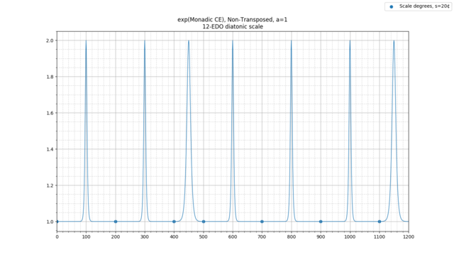
We first see the issue with our "raw" version of CE when we look at the 12-EDO diatonic scale, this time using our spiffy new plotting software:
(This is now the exp of entropy but is otherwise the same as before. Exact scale degrees are given by circles rather than x's. Looking directly at the exp of entropy is a useful measure for reasons we will go into later.)
This plot of the 1-CE of the 12-EDO diatonic scale uses all notes with equal probability. (If we instead use the Krumhansl-derived probabilities from before, we get a plot that is negligibly different.)
As we can see, there are 7 distinct minima, one for each scale degree of the diatonic scale. Maxima occur in between scale degrees; as a result, we can see that 300 cents is a maximum, being between 200 and 400 cents.
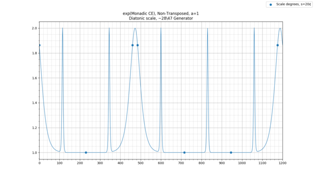
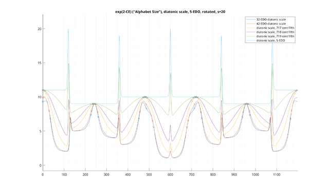
To see how this doesn't model Western music perception, look at how the diatonic scale changes as it is detuned to the extremes of 5-EDO or 7-EDO, where we previously noted the perception of the scale begins to break down. Here is a plot of the raw 1-CE of the diatonic scale generated by 715 cents (approximately 28\47):
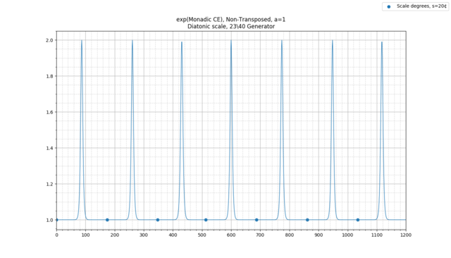
You can see that in some meaningful sense, the behavior is as expected - the major third and perfect fourth have become ambiguous, as have the major seventh and the tonic. However, things are different at the 7-EDO extreme. Consider the diatonic scale generated by 690 cents (23\40):
Previously, we noted that near 7-EDO, it becomes difficult to distinguish major and minor thirds, seconds, sixths, and sevenths, as well as perfect and augmented fourths, and perfect and diminished fifths. However, this is not shown in the above graph!
The basic issue with the above model is that we are basically treating the diatonic scale here the same way we would treat a Gamelan slendro or pelog: as an unchanging scale, with no modulation or transposition. We just have seven pitches that notes are simply matched to. This works well for Gamelan music, for instance, where you only use immovable-pitch scales and will never hear a note between two notes of the current pitch set.
In Western music, however, changes in the pitch set are quite frequent, resulting from techniques such as modulation, chromaticism, retonicizations, secondary dominants, borrowed chords, etc. As a result, the pitch set is constantly changing in subtle ways, so that there is always a chance that the transposition of the scale has changed.
The behavior we really want is to compare the incoming note to all different transpositions of the scale, not just the original chosen one. To do so, we will define the transpositionally-invariant categorical entropy.
Transpositionally-Invariant Categorical Entropy
For our raw n-adic CE, we defined the variables [math]X_n[/math] and [math]Y_n[/math]. Our mistuning/spreading function is then represented as the probability of each output tuning, given a particular choice of reference chord:
$$ P(Y_n=y_n|X_n=x_n) $$
for which the basic example is a multivariate Gaussian with standard deviation s, centered at the notes in the reference chord [math]x_n[/math].
Suppose to this, we add another random variable [math]T[/math], a continuous variable representing the number of cents the current scale is being transposed. If [math]T=0[/math], the output tuning is the same. But if [math]T=\mu[/math] for some nonzero [math]\mu[/math], then the output tuning of each note is shifted by [math]\mu[/math] cents, so that the mean of the output Gaussian is shifted by [math](\mu, \mu, ... ,\mu)[/math] cents.
Then our mistuning function becomes the probability of each output tuning, given a particular choice of reference chord and transposition:
$$ P(Y_n=y_n|X_n=x_n, T=t) $$
We can also then ask, for a particular output chord tuning and transposition, the probability that each reference chord [math]x_n[/math] generated it:
$$ P(X_n=x_n|Y_n=y_n, T=t) $$
Now, to represent the situation where we aren't sure what the transposition is, we will let [math]T[/math] be the uniform distribution on possible transpositions, e.g. the uniform distribution on cents from 0 to the equivalence interval. (This definition can be finessed for aperiodic scales, although we will not do this here.) Then we can ask about the joint distribution on chords and transpositions, given a particular transposition:
$$ P(X_n=x_n, T=t|Y_n=y_n) $$
And then, lastly, we marginalize on transpositions to ask can ask about the marginal probability for each chord given an output tuning, where all possible transpositions are taken into account:
$$ P_T(X_n=x_n|Y_n=y_n) = \int_{0}^{q} P(X_n=x_n, T=t|Y_n=y_n) dt $$
where [math]q[/math] is the equivalence interval, so will typically be 1200 cents, and the subscript [math]P_T[/math] indicates that we have marginalized on the T.
Once we have defined the above, we can redefine our transpositionally equivalent CE as:
$$ H_T(X_n|Y_n=y_n) = -\sum_{x_n\in X_n} P_T(X_n=x_n|Y_n=y_n) \log P_T(X_n=x_n|Y_n=y_n) $$
Given this, we can also define the "raw" CE as the quantity [math]H(X_n|Y_n=y_n, T=0)[/math], indicating that it is only relative to the one possible transposition of 0 cents.
Transposition-Invariance, Coordinate Change, and Dimensionality
After doing the above, all n-ads that are simply transposed versions of one another will have the same categorical entropy. For example, the chords (0, 400, 700) and (100, 500, 800) will have the same CE, as they only differ by the vector (100, 100, 100), or a constant transposition of each note by 100 cents. In general, integration on the [math]T[/math] variable above ends up "smearing" the 2D plot along the (1, 1, 1) vector (and similarly for higher-dimensional CE).
Since all transposed versions of the same chord have the same CE, we can simply take the version of each chord with the first note at "0" cents, such as (0, 400, 700) above, and then drop the first coordinate entirely, yielding (400, 700). This represents the tuning of each note relative to the lowest note in the chord.
As a result, transposition invariance reduces the dimension of the space by one, making the plots similar to the way that HE works: the transpositionally-invariant 2-CE is a 1D plot, the transpositionally-invariant 3-CE is a 2D plot, and so on. (The transpositionally-invariant 1-CE is just a single 0-dimensional scalar and hence uninteresting.)
An Important Technical Note About Scaling [math]s[/math] For Transpositionally-Invariant CE
If we are using the usual choice of Gaussian spreading function, then the above integral is simply an integral on a multivariate normal distribution. This integral yields a new multivariate Gaussian.
While we will not prove this here, it can be seen that the new Gaussian will have covariance matrix equal to [math]C=s^2(I_{n-1} + O_{n-1})[/math], where [math]s[/math] is the standard deviation parameter, [math]I_{n-1}[/math] is the [math](n-1)\times(n-1)[/math] identity matrix, and [math]O_{n-1}[/math] is the [math](n-1)\times(n-1)[/math] all-ones matrix. This skews the Gaussian along a particular axis; changing the coordinate system to whiten the Gaussian is equivalent to choosing triangular note axes for transposed 3-CE, tetrahedral axes for transposed 4-CE, etc. For those familiar with n-HE, this is exactly how the multivariate Gaussian works in that system.
The important thing about the above is the covariance matrix has determinant equal to [math]ns^{2(n-1)}[/math], which can be thought of as the "total effective variance" of the Gaussian. If we were to change the coordinate system to whiten this Gaussian (e.g. put it in triangular/tetrahedral/etc axes), the "s" value that would generate this Gaussian is scaled relative to the non-transposed version by a factor of [math]n^{\frac{1}{2(n-1)}}[/math].
In other words, if we have [math]n=2[/math], so we are looking at transposed dyadic CE, our effective value of [math]s[/math] becomes [math]s\sqrt{2}[/math]. If we're looking at transposed triadic CE, our effective value of [math]s[/math] becomes [math]s\cdot 3^{\frac{1}{4}}[/math]. For 4-CE, the effective value is [math]s\cdot 4^{\frac{1}{6}}[/math] and so on.
To be unambiguous, for transpositionally-invariant CE, we will generally refer to this as the "effective" or "total" value of s, with the original s value pre-scaling being referred to as the "raw s."
2-CE Examples, Transpositionally-Invariant
Below, all examples use the uniform distribution on the dyads of the scale.
Example: 12-EDO diatonic scale, transpositionally-invariant
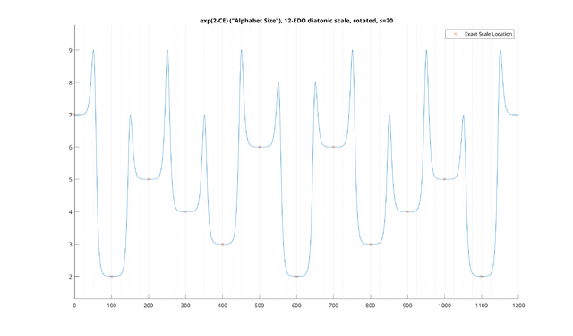
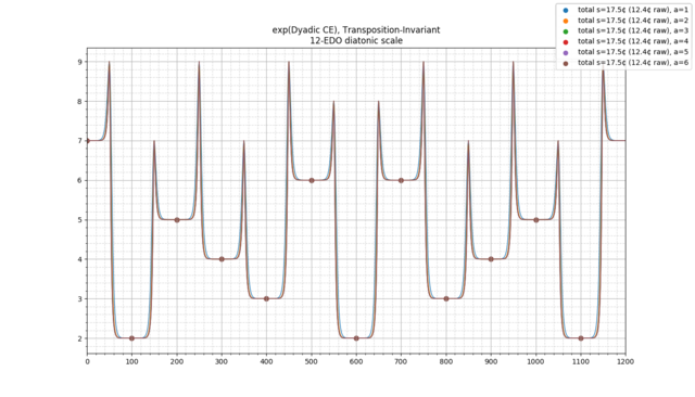
Let's look at a particular example: the transposed 2-CE for the 12-EDO diatonic scale, with uniform probabilities on each note, with a "total" s of 20 cents (or ~14.1 cents per note). We then obtain the following:
And now, we see a very different graph, representing all of the intervals appearing anywhere in the scale.
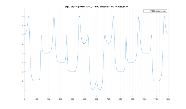
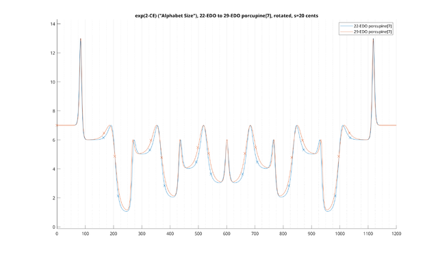
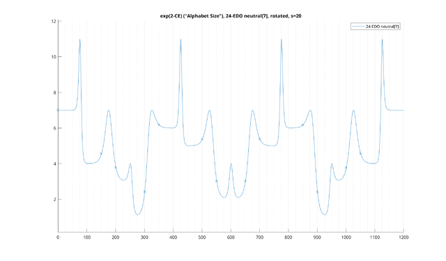
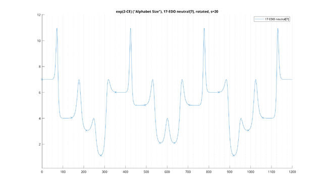
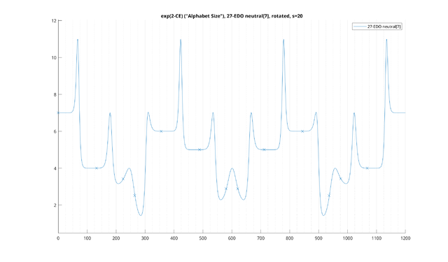
Note that above, we have not directly plotted the entropy, but rather the exponential of entropy, a quantity sometimes called "alphabet size." This is a useful quantity to look at: it quantifies how useful each interval is in telling you where you are within the scale. For uniformly distributed scales, it can be interpreted as the remaining number of possible scale transpositions consistent with your receiving that dyad as input. However, the alphabet size is much more general, and can even handle ambiguous dyads and nontrivial scale distributions, for which the same basic interpretation holds.
For example, you can see that 200 cents has an alphabet size of 5. This can be interpreted as telling you that there are five places in the diatonic scale it can appear: for example, in the major mode, it appears between the tonic and M2, the M2 and M3, the P4 and P5, the P5 and P6, or the P6 and P7. In short, in this particular situation where we are trying to match things to the diatonic scale, once we have heard a major second, we have narrowed it down to only five possible transpositions of the diatonic scale which agree with this "measurement."
On the other hand, consider the 100 cent interval, which has an alphabet size of two. The 100 cent interval "narrows things down" much more than the 200 cent interval. Once we've heard it, we know there are only two transpositions remaining.
Then, as a trivial example, you can see that for the 12-EDO diatonic scale, the 0 cent interval has an alphabet size of 7: simply playing a unison does not help you figure out at all where you are within the scale.
These examples all involve looking at notes which are within the scale, but we can also ask this question of notes that are not. For example, you can see that in this scale the 50, 250 and 450 cent intervals have an alphabet size of 9, which is even more ambiguous than one single note. This is because there is now ambiguity as to which diatonic intervals these are to begin with. For instance, it is possible that this 250 cent interval is a sharp major second, in which case there are five transpositions remaining. But, it could also be a flat minor third, which would make it four possibilities.[9] Since there's an equal chance of both at 250 cents, we have nine possibilities total. We also get a smooth curve for categorically ambiguous intervals at any point on in the spectrum, so that the alphabet size clearly generalizes the number of occurrences of the interval in the scale. This will become particularly important as we change the tuning of the generator, which we will do in our next examples: as things get close to the extremes of 5-EDO and 7-EDO, even the intervals of the scale itself will start to become increasingly ambiguous due to smearing effects in this way.
We also note that this basic metric can be interpreted several ways. For instance, if we know that we are playing some kind of "major" modality, hearing a major second narrows the possiblities down to five choices of tonic. On the other hand, we can also interpret it as though we know what the tonic is, but don't know what the mode is. Then, hearing a major second on the tonic means there are five possible modes that agree with this - Lydian, Ionian, Mixolydian, Dorian, and Aeolian - with Phrygian and Locrian eliminated. The same mathematical metric models both of these situations equally. Thus, regardless of whichever of these interpretations is musically relevant, in both situations we can clearly see that the 100 cent interval is much more useful than the 200 cent interval in "orienting" yourself within the diatonic scale.
This is, in general, how to interpret the CE for each interval in a scale: it tells you how much uncertainty is remaining in establishing the overall picture of the scale in your head once you've heard just that one interval. The lowest-CE intervals are related to what Paul Erlich calls "signposts" in his paper Tuning, Tonality, and Twenty-Two-Tone Temperament. However, note that the absolute number of the alphabet size only corresponds literally to the "number of transpositions" or "number of modes" if the intervals are given a uniform distribution, and if you are looking at an interval which is relatively categorically unambiguous. Otherwise, it is simply a scalar value which is to be interpreted similarly, as a kind of "probability-weighted number of transpositions."
We also note that the same metric can be used for scales which are non-uniform in distribution to begin with. For instance, if for whatever reason the minor third is extremely unlikely to be played in some piece of music, then the alphabet size of 250 cents would decrease, since the probability of the M2 is so much likelier than the m3 to begin with. Thus, this interval would become more effective in orienting ourselves in the scale, since we have removed an ambiguous possiblity from the scale. We will deal with this more when we talk about the "channel capacity" of the scale later.
Next, we will look at what happens to this plot as we change the tuning of the diatonic scale.
Example: 31-EDO diatonic scale, transpositionally-invariant
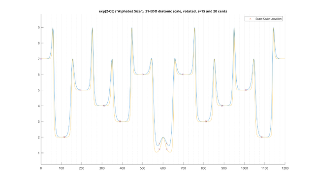
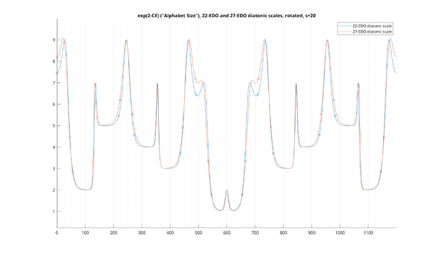
Now, let's consider a different example: the 31-EDO diatonic scale, made transpositionally-invariant. This time, we will plot the scale for "total" [math]s[/math] both at 15 cents (in blue) and 20 cents (in orange), or equivalently [math]s[/math] values of 10.6 cents per note and 14.1 cents per note, respectively:
We can see that the general shape of the curve is similar. However, the 12-EDO curve had a local minimum at 600 cents, with an alphabet size of two, corresponding to two modes (Lydian and Locrian). In 31-EDO, this interval is split into two intervals: the augmented fourth and the diminished fifth, and indeed we can see the corresponding split into two tritones in the middle of the curve.
However, we note that for total s=20 cents (blue curve), this is not enough to bring the alphabet size for each interval to 1, as you would expect - after all, in the diatonic scale, the diminished fifth and augmented fourth each appear in the scale in only one way. Instead, the alphabet size is 1.5. This is because at this value of [math]s[/math], due to "smearing" effects, the diminished fifth and augmented fourth are close enough in 31-EDO to be partly confused with one another! As a result, hearing one of those intervals does not entirely narrow the scale down to one transposition, since there is a kind of "bottleneck" in determining which interval you are hearing to begin with, hence restricting your ability to figure out which it fits into the diatonic scale. If they were completely indistinguishable, as in 12-EDO, the alphabet size would be 2, whereas if they were perfectly distinguishable, the alphabet size would be 1; the value of 1.5 indicates that we are somewhere between these two situations.
We can see that for total s=15 cents (orange curve), the situation is better: the alphabet size for each interval is 1.231.
Even more interestingly, however, we can see that the local minimum of CE is not located at the scale interval itself! That is, we can see that deliberately bending the interval by "exaggerating" the difference between the aug4 and dim5 can lower the CE, by removing the "interference" from each interval's neighbor and making it easier to figure out which interval you are hearing. We will see this theme again and again: detuning from a reference can, paradoxically, lower the CE of an interval.
Example: 19-EDO and 26-EDO diatonic scales, transpositionally-invariant
Let's continue our journey by looking at the 19-EDO diatonic scale, again with a "total s" of 20 cents (s per note = ~14.1 cents):
We get some more interesting results here: relative to 31-EDO, the augmented fourth and diminished fifth are now much easier to distinguish for the same value of [math]s[/math], each having an alphabet size of 1.276 for total s=20 cents. Furthermore, they are fairly close to their respective local minima.
However, we can see that the minor second and major seventh are beginning to creep up in CE, due to a slight increase in their probability of being confused with the major second: they now have an alphabet size of 2.164. Further, both would benefit from intentional detuning: the minor second will be less ambiguous if it is flattened, reaching a minimum of CE near 98 cents, and the major seventh will likewise be less ambiguous if it is sharpened, reaching a minimum of CE at 1102 cents - not quite enough to be the 18\19 interval, but sharper than 17\19. A similar effect is happening for the other scale intervals, to a lesser degree: from a purely categorical standpoint, the major third would benefit from bending up and the minor third from bending down.
Beyond that, we can see that most intervals are similar enough to 31-EDO. However, we get a very different picture at 26-EDO, again setting total s=20 cents:
And now we can see that the situation has decayed fairly dramatically. Most scale intervals are located somewhat far from their nearest local minima. The minor second, which should have an alphabet size of 2, now is 3.796, indicating a significant degree of confusion with the major second. The major third has increased from 3 to 4.337, indicating it is becoming confused with the minor third, which has increased from 4 to 4.964. The augmented fourth has gone up to 3.559.
We can see that each interval would benefit from a great degree of retuning: the minor second reaches a minimum at 96 cents or so, the major second at 229 cents, the minor third at 281 cents, the major third at 413 cents, the perfect fourth at 467 cents, and the augmented fourth at 582 cents. In particular, the major second is closer to the local maximum at 184 cents than the nearest local minimum!
Example: Extreme Diatonic Scale Tunings, toward 7-EDO and 5-EDO, transpositionally-invariant
Let's now consider a progression of diatonic scales, starting at 26-EDO and going to 7-EDO, again with a total s of 20 cents (s=14.1 cents per note):
We can see that, starting at 26-EDO, things degrade pretty predictably: intervals increase steadily in CE until you get to 7-EDO. They leave a "wake" of local minima behind them, so that each interval would benefit from detuning in the direction of the local minimum.
Interestingly, you can see that in a certain sense, our model "degrades gracefully" at 7-EDO (red curve): the alphabet size of each interval is equal to 7, indicating that at this point, no interval can help you distinguish between the seven modes of the diatonic scale. The general shape of the curve is relatively similar to our initial curve for 12-EDO, only with seven different categories. (Note that this is only an approximation to 7-EDO with the generator at 686 cents rather than 685.714 cents, which is why the curve is slightly distorted.)
We can get a similar effect as we approach 5-EDO. Let's start with 17-EDO, total s=20 cents:
We can see a fairly sensible curve, although this model seems to suggest slightly detuning towards 12 may improve categorical clarity of things, counter to many anecdotes suggesting that 17-EDO is superior in this regard. However, this tends to be sensitive to the value of s, and as we will see later, there is a close value of s that suggests a value close to 17-EDO for the best diatonic scale. Indeed, this common anecdote may even be useful in deciding the "correct" value of s to use.
Let's see what happens if we move to 22-EDO, and then 27-EDO:
We can see a similar degradation as we move towards 5-EDO as we did to 7-EDO: this time, the P4 gets confused with the d5, the m2 gets confused with the P1, and the M2 with the m3.
Let's go to 32-EDO and then all the way to 5-EDO:
You can see that the reference scale degrees get further from the minima as the tuning moves toward 5-EDO, and we even have a point where the reference notes are close to maxima of CE relative to themselves! At 5-CE, we again get a graceful degradation, although two of the intervals (240 cents and 960 cents) are lower in CE in that they technically enable us to distinguish between slightly more of the degenerate diatonic scales than the others.
Examples: Porcupine[7] scales, transpositionally-invariant
Let's consider some other temperaments. Consider the porcupine "spectrum" from 15-EDO to 22-EDO, with "total" s=20 cents:
We can see that for 15-EDO and 37-EDO, CE remains pretty low for the scale intervals: In particular, the "signpost" here is the large second ("L2"), which has an alphabet size of 1.052 in 15-EDO and 1.178 in 37-EDO. Likewise, the second-lowest CE interval is the large third ("L3"), which has an alphabet size of 2.027 in 15-EDO and 2.143 in 37-EDO. 59-EDO does slightly worse: the L2 is 1.473, the L3 is 2.365.
22-EDO is much worse: the L2 now has an alphabet size of 2.137, indicating the L2 is beginning to get confused with the small second ("s2") and would benefit from bending it sharp to indicate the presence of the signpost. Likewise, the L3 has increased to 2.829, indicating there is a risk of confusion with the s3. This doesn't mean that 22-EDO is necessarily a "bad" porcupine tuning, but that more care is needed to treat these potential sources of ambiguity when playing.
We can see things degrade considerably when moving from 22-EDO to 29-EDO, as shown in this curve:
From this, we can see that while 22-EDO indicates the intervals are beginning to move away from their minima and increasing in alphabet size - though not in an unsalvageable way - the situation is so degraded by 29-EDO that the intervals are near CE maxima. This indicates that 29-EDO will be much more ambiguous than 22-EDO (and indeed it is much closer to 7-EDO).
Examples: Neutral[7] scales, transpositionally-invariant
Let's try another example: the neutral[7] MOS, first tuned to 24-EDO, with total s at 20 cents (14.1 cents per note):
We can see, right away, that neutral[7] has some ambiguities in 24-EDO for this value of [math]s[/math]. The minor third is relatively far from its nearest local minimum; it should be the unique "signpost" interval with an alphabet size of 1, but instead is 2.426. Likewise, the half-sharp fourth, which should have an alphabet size of 2, is increased to 3.024. The neutral and major second are also both somewhat higher in CE than their nearest local minimum.
This isn't terribly unexpected, given that we have used the same value of [math]s[/math] from before, but have moved from the diatonic scale to neutral[7], where the chroma is only half as big. In general, in this tuning for neutral[7], we can see that the neutral third will sometimes be confused with a "sharp minor third" and vice versa, the neutral second will sometimes be confused with a "flat major second" and vice versa, and so on. Of course, it is certainly possible that ear training with this tuning system could lead to a lower value of [math]s[/math] being more appropriate.
In comparison, let's look at 17-EDO, same value of total at = 20 cents:
We can see right away that 17-EDO corrects most of these deficiencies. The alphabet size of the minor third is 1.133, fairly close to 1. The half-sharp 4 has an alphabet size of 2.1, fairly close to 2. The chroma has been increased in size from 50 cents to 71 cents, so the distinction between many of the ambiguous interval pairs above has been accentuated. Every interval is very close to its local minimum, meaning that we are near a nice equilibrium where detuning doesn't help decrease CE.
Let's now look at 27-EDO - or rather, a "quantized" version where the generator is exactly 356 cents:
We can see that many of the troublesome intervals cleared up by 17-EDO remain clear with our 356 generator, since the formerly "quarter-tone" sized chroma is now 92 cents. On the other hand, we have new ambiguities arising from that the minor second is now only 40 cents. As a result, the minor third at 264 cents is now fairly close to the major second at 224 cents, and is much increased in CE relative to its nearest local maximum, similarly to the situation with the superpyth diatonic scale. Likewise, the half-sharp fourth is now 580 cents, close enough to be confused with the half-flat fifth at 620 cents.
Examples: Tetracot[7], transpositionally-invariant
A more interesting example arises with tetracot[7]. Let's first try the 176 cent generator, which is simultaneously a rounded off version of the 34-EDO and 41-EDO tetracot generators, close to the 5-limit POTE, with total s = 20 cents (14.1 cents per note):
Right away we can see there is a lot of ambiguity. Not only are the intervals far from their minima; they are near their maxima! This is because tetracot's generator of 176 yields a chroma of 32 cents. The large step is 176 cents and the small is 144 cents. The large third is 352 cents, whereas the small third is 320 cents; likewise the small fourth is 496 cents, and the large fourth is 528 cents. These are all close enough to be easily confused with one another, at least assuming a s=20 cents.
We can try moving away from the POTE to improve categorical clarity. If we move to 27-EDO, things get noticeably better, but not quite:
While the intervals are still relatively ambiguous, they are much less so than before; each interval is much closer to a local minimum. Of course, intonationally, 27-EDO is much less harmonic than 41-EDO, but we gain the benefit of being more easily able to distinguish between the notes in the scale.
We can go even further toward 20-EDO:
We can see things are much better from a categorical standpoint: it is much easier to distinguish the notes of the scale from one another. Things aren't perfect, but each interval is relatively close to a local minimum. Of course, 20-EDO is a fairly rough tuning for tetracot, relative to what it is capable of - the 3/2's are now 720 cents, and the 5/4's are 420 cents - but we are only evaluating this one property of how distinguishable the scale intervals are from one another, not anything about the intonation.
Tetracot thus provides us with an interesting example of a harmonic/categorical tradeoff: tunings with better intonation are less categorically distinct, and tunings with better scale "clarity" have worse intonation. This gives us an interesting example of how categorical and harmonic constraints need not always be compatible with one another.
3-CE Examples, Transpositionally-Invariant
All examples use the uniform distribution on triads, and are plotted using python's matplotlib "tricontourf" plot. Different contours can be thought of as denoting different "regions."
These all have total s=15 cents (11.4 cents per note), so slightly less than the 2-CE examples.
Examples: Diatonic Scale, 3-CE, Transpositionally-Invariant
If we add transpositional-invariance to 3-CE, we get a 2D plot. Using Python's matplotlib contour plotting yields the following for the 12-EDO diatonic scale, for total s=15 cents:
Darker values on this graph (such as purple) indicate lower 3-CE, whereas brighter values (such as real) indicate higher 3-CE. The red dots are the reference triads.
The x-axis indicates the size of the first dyad in cents from the lowest note, and the y-axis indicates the size of the second dyad in cents from the lowest note. Although this is not plotted explicitly, the line going from bottom-right to upper-left is the size of the remaining dyad. (This would be better if plotted with triangular coordinates, but I'm not sure how to do this in matplotlib.)
As expected, and similarly with 2-CE, you can see that triads containing the tritone are generally lower in transpositionally-equivalent 3-CE, showing that they yield a lot of information about where in the scale. Note also that the chord (400, 1000) (e.g. P1-M3-m10) is also low in CE, since it uniquely shows you where you are in the scale. The chord (500, 700) (e.g. P1-P4-P5) is higher in CE, since it doesn't give much info about where you are in the scale.
Let's see how things change for 31-EDO:
First, while it looks like the entire graph has gotten lighter (and hence higher in CE), this is simply a result of the scaling of matplotlib's tricontourf routine. However, you can see that the triad formerly at (600, 600) has now split into two regions, that the triads are still generally near local maxima.
Now let's look at 19-EDO:
Again, the graph looks lighter in general, but this is simply a result of the scaling. This plot is similar to the last, but you can see that there are now two very distinct regions at (568, 568) and (631, 631). Likewise, you can see that the triads have begun to shift towards the edge of their regions.
This effect gets more prominent at 26-EDO:
And now you can see that the triads are fairly far from their nearest local maxima, indicating that the triads of this scale have become more ambiguous and would even benefit from detuning.
Similarly we can look at 17-EDO:
You can see most triads have shifted somewhat from the midpoint of each region, but are still within the same contour (and hence relatively close to local minima).
Examples: Mavila[7], 3-CE, Transpositionally-Invariant
Let's try mavila[7] now. 16-EDO, generator 675 cents, total s=15 cents (11.4 cents per note):
We can see this is a fairly nice tuning, from a categorical standpoint. All triads are located at the midpoints of their regions, and things seem fairly clear. Triads containing the 450 cent interval are very low in CE as they uniquely indicate where you are in the scale. So do the augmented chords (375, 750) and (375, 825), both of which contain a 450 cent interval. Chords like (225, 675) and (225, 750) are useful to find your position as well.
We can also look at the 678 cent generator, or ~23-EDO:
We can see that things have shifted somewhat, although perhaps not terribly badly. 23-EDO is more ambiguous than 16-EDO; triads are closer to the edges of their regions, but not necessarily badly enough to break down scale perception.
Rather than continuing towards 7-EDO, we can also go towards 9-EDO. Let's first look at a generator of 672 cents, or 25-EDO:
We can see that things for 25-EDO have shifted relative to 16-EDO, similarly to how they did for 23-EDO, although in a different way. The 25-EDO triads are, similarly to 25-EDO, pushing up to the edges of their regions, although not necessarily enough to be really ambiguous.
We can continue along the spectrum and look at a very flat 670 cent generator, close to ~24\43:
And now we can see things have gotten significantly ambiguous: chords are converging on one another, and are often beyond the contour of the region of the nearest minimum.
Lastly, we can look at a generator of 667 cents, or a rounded-off 9-EDO:
And now we can see that the ambiguous chords have "converged" into one another, so that we have neat regions again. However, although the plot doesn't show this due to the way it is scaled, although the triads are near the midpoint of each region, the regions are usually higher in CE as there are different competing "enharmonically equivalent" versions of each triad, so that hearing a triad doesn't necessarily narrow down where you are in the scale as much as it did in 16-EDO.
For example, in 16-EDO, the triad (225, 675) or (L2, P5) had an alphabet size of 1, as it uniquely showed you where you are in the scale. However, in 9-EDO, the same (L2, P5) triad is tuned (267, 667), which is the same as (m3, P5), for example. As a result, there are more matching places in the scale where a (267, 667) triad could occur (since it is also a minor triad), so the CE is higher.
Examples: Porcupine[7], 3-CE, Transpositionally-Invariant
Let's look at Porcupine[7] as well. Let's look at 15-EDO (generator 160 cents) with total s=20 cents (11.5 cents per note):
You can see each reference triad is at the midpoint of its own region, and that chords containing the rare 240 cent interval are generally lower in CE than the rest (as the 240 cent interval tells you where in the scale you are). For example, the (240, 720) triad (mapped as 1/1-9/8-3/2) is one such triad with an alphabet size of 1, telling you uniquely where you are in the scale.
Let's look at porcupine[7] with generator 162 cents, close to ~37-EDO:
We can see the regions for each triad have changed somewhat, but the reference triads are still placed close to the minimum of each region.
If we go to a 163 cent generator, close to ~59-EDO, we get:
And now we can see that the regions and triads have shifted so that triads are pushing up to the edge of their regions, but are still well within the contour.
Once we go to a generator of 164 cents, or approximately 22-EDO, we then get this:
And now we can see that some ambiguity is beginning to enter into the picture. Triads are near the edge of their regions, although not necessarily ambiguous yet. Many triads would benefit from some deliberate "bending" to enhance categorical clarity in identifying scale position, away from the reference: e.g., bending the ~216 cent L2 sharp, bending the ~380 cent L3 sharp, bending the ~328 cent s3 flat. However, all things considered, while things are "ambiguous-ish" here, they are not necessarily totally ambiguous.
To see something very ambiguous, we can increase the generator to 166 cents, approximately ~29-EDO:
And now we can see that triads are very much at the edges of their regions, sometimes even past the contour enclosing the nearest local minimum. As the tuning gets closer to 171 cents (7-EDO), this increases.
Detuning Enhancement Principle and Scale "Categorizability"
The examples above bring an important realization: for some scales, the CE of each interval can actually be enhanced by bending the interval away from its usual position. For these scales, bending the note in question can sometimes have the effect of enhancing the sense of category by bringing it away from ambiguous competing intervals.
A good example is meantone[7] in 19-EDO (given above). This model predicts the leading tone would be enhanced if it were sharpened, by enhancing the categorical distinction between it and the minor seventh. Values of s between 15-25 cents typically put the maximum between the leading tone of 12-EDO and 17-EDO. This suggests that flexible-pitch instruments would gain some categorical clarity by sharpening the leading tone in 19-EDO slightly.
Another example is porcupine[7] in 22-EDO (also given above). In this situation, the large second is 216 cents and, for s=20 cents, tends to be confused with the small second at 164 cents. You can see, however, that by bending the large second toward 240 cents, the CE is lowered significantly. This suggests that flexible-pitch instruments would benefit from sometime bending the large second upward slightly, to accentuate the impression of the L2 being a "large" second in the scale.
The ability of this model to suggest which intervals should be bent to enhance clarity can lead to interesting results. For example, in 24-EDO neutral[7], this suggests that the minor third would benefit from enhanced clarity if bent toward 274 cents, where there is less interference from the neutral third. However, this model also suggests that the neutral second should be bent toward 100 cents. This is because there is no 100 cent interval appearing anywhere in neutral[7], so this model presents no conflict.
However, intuitively, we may want to include this interval for comparison, as well as other intervals not in neutral[7] but in its MODMOS's (such as the "Rast"-ish MODMOS of LnnLLnn or the diatonic scale). One way to do so is by taking the union of the different modes of both scales. For example, in 24-EDO below, if we mix the modes of Rast and the diatonic scale, we get:
You can see the model now predicts a categorical enhancement from bending the neutral second slightly flat to 144 cents, as does bending the major second slightly sharp to 222 cents, and bending the major third sharp to near 413 cents.
While this is certainly a simple model, it does seem to give useful guidance on how to bend intervals for melodically expressive purposes, often yielding different results than bending for purely harmonic purposes. For future work, it would certainly be interesting to see what it suggests, for example, if we were to put in a list of authentically-tuned maqamat from some region and pit them against one another: would the suggested bends be similar to those commonly used?
The above examples bring us to another main realization: some scales have their own intervals ranking so high in CE that they almost become maxima. This tells us that such scales are, in some sense, difficult to categorize: intervals will get confused with one another frequently, or even appear to blur together. A good example is tetracot in 41-EDO (shown above).
These scales are, of course, still musically useful - indeed, intervallic ambiguity can be very musically beautiful. These scales simply require a different musical approach than scales where the intervals are all low in CE and distinct from one another. They may need to use more musical context to aid in distinguishing ambiguous intervals from one another. They may require a more careful use of modulation, or a more careful treatment of ambiguous intervals in general, so as to avoid confusing the listener regarding which scale degrees are being played. Or, a composer could simply embrace the ambiguity as a feature of the music.
This leaves us with a question, however: rather than look at the categorical entropy of individual intervals, can we obtain some notion of the categorical entropy of a scale? We will see below that we can, using Shannon's concept of "mutual information."
Categorical Mutual Information of a Scale
NOTE: As before, this can get pretty technical, so you may want to just skip ahead to the examples.
Intuitively, we want to get some sense of the "total" categorical entropy contained in a scale, relative to itself. Are the scale's own intervals low in CE, relative to itself as a reference? Are the peaks of CE located reasonably far from the scale's intervals, near the midpoints? While there are a few ways to quantify this, for our purposes the best will be the "Categorical Mutual Information", or CMI, introduced by Keenan Pepper, which is the Shannon mutual information of the random variables [math]X[/math] and [math]Y[/math].
Before we define the CMI, we will define a simpler metric to gauge the total categorical entropy of a scale: the weighted average of the CE for all possible intervals, relative to that scale, weighted by how likely the interval is to be played.
Preliminaries: Average Categorical Entropy of a Scale
The Average Categorical Entropy (ACE) of a scale is defined as the expected value of Categorical Entropy. In Shannon's terms, this is called the "conditional entropy", and is notated [math]H(X|Y)[/math].
The ACE is defined as the quantity:
$$ H(X|Y) = \mathbf{E}\left[H(X|Y=y)\right] $$
where the expectation is taken on all values of [math]Y[/math]. The ACE is likewise defined similarly for n-adic CE, and for transpositional-invariance, although we will simply refer to the monadic [math]X[/math] and [math]Y[/math] variables here to keep the description simple.
Now, while [math]Y[/math] is in theory supposed to be a continuous random variable, we will find it is usually a lot easier to deal with information theory if we use discrete random variables on a finite set. So, we will instead quantize [math]Y[/math] to a set of discrete cent values within a specified range and with a sufficiently small step size: for example, the set of all intervals between 0 and 1200 cents, with a step size of 1 cents or 0.1 cents.
If we use this simplification for [math]Y[/math], we obtain the following:
$$ H(X|Y) = \sum_{y \in Y} P(Y=y) H(X|Y=y) $$
In this expression, [math]P(Y=y)[/math] represents the probability of [math]y[/math] being played as an output interval for *any* reason, as a smeared version of *any* input category. Since [math]H(X|Y=y)[/math] is the categorical entropy of the arbitrary interval [math]y[/math], this gives us an expression for the weighted average of the CE of all intervals.
Note that the probability distribution on [math]Y[/math] is not arbitrary here, but is derived directly from our original definitions of [math]X[/math] and [math]Y[/math]. We simply place Gaussians centered at each interval [math]X[/math] in [math]X[/math], scaled vertically by the probability on [math]X[/math], and add them together. This can be formalized by a combination of the conditional probability chain rule and the definition of marginal probability, which we will not derive here.
To visualize this for the 12-EDO diatonic scale, for instance, we obtain the following:
The top curve is the exp-CE (alphabet size) of every interval in the 12-EDO diatonic scale, showing how frequently they are played on average in the scale (assuming a uniform distribution on intervals and transpositional-invariance). The middle curve gives the Gaussian spreading function for each interval. Lastly, the bottom curve gives the output probability for [math]P(Y=y)[/math].
You can see in the bottom curve that, as expected, the generators are played most (500 and 700 cents), and the half step and half-octave played least (100 and 600 cents). So the intervals that are most likely to be played are, in general, the intervals of the scale, with a slight Gaussian-shaped "halo" of intonational possibilities around each one, weighted by the probability of each interval and how commonly it occurs.
Once we have the above, we can easily compute the conditional entropy [math]H(X|Y)[/math]: simply take the log of the top curve, multiply pointwise by the bottom curve, and sum the whole thing.
ACE has a very clear, precise interpretation, both musically and information-theoretically: it quantifies how much uncertainty there is, on average, in determining what scale degree is being played upon hearing a real-life realization of a note from that scale (with some slight possible mistuning). For scales that score low on this metric, hearing a average note from the scale being played is sufficient to eliminate most of this uncertainty, so that there aren't many competing interpretations of the note. Scales that score higher, on the other hand, will have more uncertainty on average, so that you are more often left guessing whether it is a detuned version of this or that reference note. These types of scales will require different musical techniques to narrow down the ambiguity further, such as using musical context to help in distinguishing the possibilities.
A Better Model: Categorical Mutual Information
The main issue with using ACE is that it always scores smaller scales higher, since there are less notes in general and hence less to compete with one another. While this is useful for distinguishing between different tunings of the same MOS, for instance, it also always thinks that a scale with just one note is the greatest scale in the world, since there is always only one possibility and hence never any uncertainty at all. Certainly, an ambiguous scale will be unsuccessful at transmitting musical information, but so will a scale that doesn't contain any information at all.
The simple way to balance these requirements is to reward scales that manage to successfully squeeze in more notes without creating ambiguity. This means we should also be looking at how much information is contained in the original scale to begin with, before any detuning is added. This is best quantified by looking at the entropy [math]H(X)[/math] of the scale as a random variable. In this situation it may be more intuitive to interpret this quantity not as "uncertainty," but rather the "informational potential" of the scale, before any detuning or smearing. (It may be helpful to think of this as a probability-weighted version of the scale size, or rather its natural logarithm.)
Given that, we would like for our scale to perform better if the original scale information [math]H(X)[/math] is high, and to perform worse if the average categorical entropy [math]H(X|Y)[/math] is high. The simple thing to do is subtract the latter from the former, yielding Shannon's famous "mutual information" quantity, denoted by [math]I(X;Y)[/math]:
$$ I(X;Y) = H(X) - H(X|Y) $$
This is the Categorical Mutual Information of the scale, which Keenan Pepper first suggested using. This quantity tells us, on average, how much information about the notes of a scale you get from hearing someone play it.
Interpretation
We can think of this as modeling a process whereby the scale begins with some degree of initial entropy, representing the set of musical possibilities that might be played. Once you hear a note, these probabilities collapse into a particular musical outcome. This is represented by an entropy reduction, or a decrease in uncertainty.
If the scale is 100% unambiguous, this is basically what happens: there is a total entropy reduction, so that hearing a note played unambiguously determines the interpretation. If the scale is muddy, however, there will only be a partial entropy reduction, since there will tend to be a few competing interpretations for the note you just heard. This tells you that hearing a note from the scale isn't necessarily sufficient to determine an unambiguous musical outcome.
This latter situation leads to a "bottleneck" on [math]I(X;Y)[/math] as notes blur together and become indistinguishable. This leads to a very nice interpretation, in particular for the exponential of musical information: it is the "effective number of intelligible notes" in the scale, which can be much less than the true number of notes in the scale if it is muddy and things blur together. (This interpretation must be taken more loosely if the probability on the scale is not a uniform distribution, or if transpositional-invariance is used, but it is still a good starting point.)
The mutual information is often used in information theory to quantify how "dependent," "related," or generally "connected" two random variables are, by measuring how much information from one tells us about the other. Typically, [math]X[/math] and [math]Y[/math] are considered the input and output of a noisy channel. In that situation, a low mutual information means the noise has almost entirely decoupled the input and output from one another, in that you never quite know which output symbol you'll get for a certain input, or know which input symbol created your measured output. A high mutual information is basically desirable in this situation, since it means the output is usually predictable from the input and vice versa. Even though we are using this in music rather than communications, we have basically the same situation, so this is a useful quantity to look at.
Another Definition for Categorical Mutual Information
The mutual information has some useful mathematical identities. For example, it is well-known that the mutual information is always symmetric. That is, we have
$$ I(X;Y) = I(Y;X) $$
We can use this to get a different definition for the mutual information (originally suggested by Keenan Pepper), which we will later find useful:
$$ I(X;Y) = H(Y) - H(Y|X) $$
where [math]H(Y)[/math] is now the entropy of the output variable, and [math]H(Y|X)[/math] is the conditional entropy of tunings given a choice of note.
A Simplification For Identical Tuning Curves
Given the above, we note that assuming we are using the same detuning curve for each note -- e.g. a Gaussian with some standard deviation [math]s[/math] -- the quantity [math]H(Y|X)[/math] is a constant that does not depend on the choice of scale [math]X[/math]. Furthermore, this holds even if we are not using a Gaussian, but rather some arbitrary detuning curve that is identical for each note other than the mean. We can see this by looking again at the definition of conditional entropy:
$$ H(Y|X) = \sum_{x \in X} P(X=x)H(Y|X=x) $$
so we simply have a weighted sum of entropies [math]H(Y|X=x)[/math] for all notes in [math]X[/math].
Each entropy [math]H(Y|X=x)[/math] is the entropy of the probability distribution [math]P(Y|X=x)[/math]. However, assuming we are using identical tuning curves for each note, whether Gaussian or otherwise, these probability distributions are all translated versions of one another!
Since translating does not change the entropy, we know that every single [math]H(Y|X=x)[/math] is identical for all [math]x[/math]. So we have the result:
$$ H(Y|X=x) = H[G_s] $$
where [math]H[G_s][/math] simply denotes the entropy of the detuning curve, taken as a point-spread function.
As a result, the conditional entropy can be rewritten as
$$ H(Y|X) = \sum_{x \in X} P(X=x)H[G_s] $$
but we know that [math]H[G_s][/math] is identical for all [math]x[/math]. So we can take this out of the summation to obtain
$$ H(Y|X) = H[G_s] \sum_{x \in X} P(X=x) $$
and lastly, since the sum of all probabilities in [math]X[/math] must be 1, we have:
$$ H(Y|X) = H[G_s] $$
So lastly, we have the result for the mutual information:
$$ I(X;Y) = H(Y) - H[G_s] $$
Now, we only really care about finding relative maxima or minima, and not the absolute value of the curve. Thus, we don't really care if the mutual information is shifted up or down by a constant. As a result, we have the following:
$$ exp(I(X;Y)) \propto exp(H(Y)) $$
that is, exp-MI is proportional to exp-output entropy.
As a result, for a given value of [math]s[/math], the mutual information is entirely determined by [math]H(Y)[/math], the entropy of the output. As we will see, this is an easy quantity to compute, as well as easy to generalize to things like the Rényi entropy.
[math]H(Y)[/math] can be viewed as a measure of how much of the pitch spectrum your scale tends to use, including mistuning effects. In a clear scale, the point spread functions for each note will tend to be located far enough apart from one another that each interval has its own unambiguous "bandwidth," leading to a high value of [math]H(Y)[/math]. In a muddy scale, the point spread functions for each interval will tend to be located on top of one another, so that it is difficult to distinguish intervals from one another, leading to a low value of [math]H(Y)[/math]. If a scale has an unused portion of the spectrum, adding another note will increase [math]H(Y)[/math], as long as it doesn't cause interference with other notes. We will see examples of this below.
n-CMI and Transpositional-Invariance
Since we have defined our CMI in terms of the average categorical entropy, we can likewise define a CMI for dyadic, triadic, or in general n-adic CE. We simply extend our previous definition to the case of random variables representing n-adic chords:
$$ I(X_n;Y_n) = H(X_n) - H(X_n|Y_n) = H(Y_n) - H(Y_n|X_n) $$
Likewise, we can get transpositional-invariance by doing the exact same thing we did previously with our new variable [math]T[/math], which we can marginalize on to get the transposed categorical entropy:
$$ I_T(X_n;Y_n) = H_T(X_n) - H_T(X_n|Y_n) = H_T(Y_n) - H_T(Y_n|X_n) $$
where [math]H_T[/math] represents the transpositionally-invariant entropy, as defined previously.
Comparing (Monadic) CMI, ACE, and Output Entropy: EDOs, 1 to 50
Let's start by looking at these metrics for EDOs. Below is a plot of CMI ([math]I(X;Y)[/math]), ACE ([math]H(X|Y)[/math]), and output entropy ([math]H(Y)[/math]) for EDOs from 1-49, for comparison:
On the left is the exp of CMI, which can be viewed as the "effective number of notes" in the scale. Note that for this plot, higher values are better, so this is different from the way CE works. You can see that for each value of [math]s[/math], as the EDO is increased, the CMI steadily increases, but asymptotically approaches a point where adding more notes doesn't add any more mutual information; you have reached the "maximum effective EDO" for that value of [math]s[/math]. Increasing the value of [math]s[/math] increases the maximum number of effective notes in the scale. This maximum value is given for different values of s (annotated in the lower right).
In the middle is the exp of ACE, the weighted average CE of the scale. Unlike the plot on the left, higher values are worse in this plot. As you can see, the "best" scale in this plot is always 1-EDO, which is always totally unambiguous no matter what the value of [math]s[/math]. This is one way to see the difference between CMI and ACE: CMI tells you how much total information a noisy scale can transmit (on average), whereas ACE only tells you how much ambiguity is in a scale.
On the right is the exp of the output entropy [math]H(Y)[/math], where greater values again denote a better score, similarly to the first plot. Since the CMI is equal to [math]H(Y) - H(Y|X)[/math], and since [math]H(Y|X)[/math] is a constant that depends only on the value of [math]s[/math] (assuming identical Gaussian mistuning curves), each curve in this plot is a vertically shifted version of the corresponding curve in the left plot with the same value of [math]s[/math].
Using the "Maximum EDO" to Choose [math]s[/math]
The above shows us that with the CMI, as you increase the number of notes in the scale, eventually you get to a point where adding more notes doesn't add any more information. Where this happens depends only on the value of [math]s[/math].
One way to view this is that, given a musical scale, listeners can only perceive some maximum number of notes as distinct musical entities before the scale simply gets too "crowded" and the threshold of ambiguity is reached. Beyond that point, increasing the number of notes in the scale does not increase the effective number of "symbols" in the mind of the listener, but rather the listener begins to chunk different notes together into different intonations of the same "symbol."
It is, of course, certainly true that every listener will vary as to how many distinct notes they can mentally represent before they begin to inadvertently confuse them as different tunings of one another. It is likely, for example, that students of Middle Eastern music will be able to cognize more notes as distinct entities than students of Western common practice music. It is also likely that people in the modern xenharmonic or microtonal community will be able to push this ability to new heights, by deliberately ear training a set of intervals with even smaller tuning deviations, and associating an entirely different set of harmonic, modal, or generally musical settings for each interval or chord in question. This variance is represented in our [math]s[/math] parameter: better pitch discrimination is represented by a smaller value of [math]s[/math], which leads to a larger maximum EDO value before things become asymptotically flat.
Furthermore, while CMI and output entropy yield the same curves - just vertically shifted - the CMI is unique in that the raw value of the exp-CMI can be thought of as representing the "effectively intelligible number of notes" in the scale. As you can see, for each value of [math]s[/math], this leads to a different asymptote for each curve, which can be interpreted as the largest possible EDO that is perceptible with that value of [math]s[/math].
Indeed, these asymptotes can be a good way to choose the desired value of [math]s[/math]! This really should be fairly intuitive: if you want to distinguish each note correctly in 12-EDO, you only need to be able to correctly process notes within a +/- 50 cent radius of the desired tuning. However, if you want to distinguish each note correctly in 24-EDO, you need twice as much precision, and now notes can only differ within +/- 25 cents. For each desired EDO, we can choose a value of [math]s[/math] so that this is the maximum possible EDO.
As you can see, for [math]s[/math]=20 cents, the maximum EDO is approximately 14.52 EDO, whereas for [math]s[/math]=15 cents, the maximum EDO is approximately 19.36 EDO, and at [math]s[/math]=10 cents it's approximately 29 EDO.
There is a useful rule of thumb to convert values of [math]s[/math] to an approximate maximum EDO [math]m[/math], assuming our interval of equivalence is [math]i_e[/math]:
$$ m \approx \frac{i_e}{4s} $$
This is derived by assuming we want our Gaussian to be such that two standard deviations from the mean equals half the distance to the next note. So if our equivalence interval is 1200 cents, this becomes:
$$ m \approx \frac{300}{s} $$
Some examples:
For [math]s[/math]=20, we get [math]m[/math]=15-EDO
For [math]s[/math]=15, we get [math]m[/math]=20-EDO
For [math]s[/math]=10, we get [math]m[/math]=30-EDO
These are all within ~1 cent of the measured values.
Of course, in real life, musical context can often make it easier to distinguish between notes. However, despite this, we regard the [math]s[/math] parameter as a good basic way, on average, to adjust the tendency to "lump notes together" vs "distinguish between them" within the model. More importantly, even if the exact cents or EDO values suggested by the model above are not perfect, one can still adjust the value of [math]s[/math] either way to obtain different curves that may be better suited toward the way that one hears.
Lower [math]s[/math] is not "Better"
An important caveat, which is one of the basic tenets of the model: we consider the value of [math]s[/math] to be a "dynamic" quality that can and should change, even in the same listener, when listening to different music in different tunings. A lower value of [math]s[/math] is not "better," nor does it indicate "superior" hearing.
A lower value of [math]s[/math] simply represents a style of hearing which is tuned to recognize a smaller range of tuning deformations as being different tunings of the "same note." This is good for styles of music with lots of notes that may be tuned closely together, yet are truly "different notes" with distinct musical purposes, and in which there is less tolerance for mistuning before things sound like "different" notes. A good example would be microtonal music in which the emphasis is on distinguishing the different musical purposes that different simple JI intervals can have, even if those intervals are tuned fairly closely to one another, perhaps played on something like a harpsichord.
A higher value of [math]s[/math] represents a style of hearing which is tuned to recognize a smaller set of notes within a larger range of tuning deformations. This is better for styles of music that involve "more bending" and "less notes." For example, real-world 12-EDO performances virtually depend on listeners being able to render the notes intelligible even if they are detuned on purpose, as in barbershop music, or even more so with blues, or played slightly out of tune, etc. In a microtonal setting, a good example would be a novel style of music with lots of note bending in some low-numbered EDO, for example something like a "14-EDO blues," where the emphasis is on recognizing tonal note "meanings" even as they are bent. Another example would be a style of music in which different JI intervals are used dynamically to enhance the harmonic intonation of a smaller set of conceptual notes which have some musical meaning on a different tonal level, perhaps like a "barbershop porcupine." In these situations, the listener will not be able to understand the music if they cannot correctly understand the meaning even if the tuning is distorted, so a larger [math]s[/math] is necessary.
An interesting real-world example is Middle Eastern maqam music, which tends to use more notes and more note bending. Middle Eastern music students learn both a larger set of core notes, but also to correctly identify them through a wider range of melismatic tuning variations, both of which would seem to influence [math]s[/math] in opposite directions.
Despite these nuances, we would still guess that even in this musical setting, there is some value of [math]s[/math] is "good enough" to yield decent results for this model in the eyes of maqam musical practitioners. This would be a worthy thing to study! As a first guess, we would think that given the two competing effects, the appropriate value of [math]s[/math] would still be lower than that of Western common practice music.
Raw Monadic CMI: Maximized at Low-Numbered EDOs (Probably)
Let's look now at the raw monadic CMI for the diatonic scale, keeping in mind this is not transpositionally-invariant, with uniform probabilities on everything:
Again, remember that higher values are now better. Note that for monadic CMI, the diatonic scale becomes ambiguous only as it gets to 5-EDO, but does not get ambiguous at 7-EDO. Rather, the monadic CMI is maximized at 7-EDO!
If you think about it, this makes sense: we are only looking at the monadic CMI, without any transpositions, modulations, etc. At 7-EDO, the notes are spaced maximally apart from one another, so ambiguity is minimized. (Of course, this simply tells us that for many musical purposes, we really want the transpositionally-invariant 2-CMI, so that we end up comparing the modes of the scale to one another as well.)
Let's also look at the raw monadic CMI for the chromatic scale:
Likewise, we can see that the monadic CMI for the chromatic scale is maximized at 12-EDO, or a generator of exactly 700 cents. This is again unsurprising, as 12-EDO again spaces each note maximally apart from one another, so that each note has as little ambiguity as possible for the same value of [math]s[/math].
This leads to an important principle: low-numbered EDOs appear to maximize monadic CMI. While this is only a conjecture for now, it seems to be clearly true; all MOS's seem to exhibit the same behavior in that monadic CMI is maximized when the notes are evened out to yield an EDO. (This is probably easy to prove by noting that CMI is maximized when output entropy is, and output entropy is maximized as the output gets closer to a uniform distribution, for which the closest point is when the notes are equally spaced.)
Lastly, note also that at 7-EDO, the value of exp-CMI is 7, at 5-EDO, the value is 5, and in between, the curve slopes to 12. This tells us that CMI degrades nicely at extremes. Importantly, this tells us that even if we add "dummy notes" tuned to the same tuning as other notes, this does not change the CMI at all. For example, at 7-EDO, the chromatic scale technically has 12 notes, but with multiple notes tuned to the same 7-EDO tuning. However, the exp-CMI value is 7, and furthermore increases smoothly from 7 as the scale is slowly detuned from 7-EDO. So our measure does seem to correctly tell us the "effective number of notes" in a scale, such that if you add identical notes at the same tuning, it does not change the CMI.
Of course, what is much more useful is to look at the transposed dyadic CMI, which will enable us to evaluate different MOS tunings. Let's do that now:
Examples: 2-CE MOS Spectra, Transposed
Diatonic Scale, 5-EDO to 7-EDO
Here's the 2-CMI of the diatonic scale, with transpositional invariance, assuming uniform probabilities on everything:
Below are the "best" tunings of the diatonic scale for each value of [math]s[/math], along with the (not-exp) CMI:
Best: 705.0 = 3.5038 (s=10)
Best: 704.4 = 3.4973 (s=12.5)
Best: 703.6 = 3.4783 (s=15)
Best: 698.0 = 3.4511 (s=17.5)
Best: 699.3 = 3.4190 (s=20)
So we can see that when values of [math]s[/math] are relatively coarse, for instance 17.5-20, the best tuning is close to 12-EDO. However, below this, for values of [math]s[/math] near 10-15 cents, the best tuning of the diatonic scale is in the 703-705 cent generator range.
Many people commonly report a preference for a diatonic scale generator that is slightly sharp of 12-EDO, with the 17-EDO generator of 705.9 cents being a fairly common choice; this is not far from the generators being reported for low-medium values of [math]s[/math] here. Although not plotted here, the maximum seems to "flip" from 12-EDO to a sharpened generator below s=16 cents, where the maximum is 703.1 cents (or approximately 29-EDO). In Paul's terms for HE, this would be close to an s of 0.93%, fairly close to the standard suggested value of s=1.0%, or 17.22 cents.
Note again that at the extremes or 5 and 7-EDO, the exp-2-CMI is 5 and 7, indicating, as expected, an "effective number of notes" of 5 and 7. However, note that in between, the effective number of notes may not be exactly the same as expected; for example, the max exp-CMI attained for s=10 is 11.3435. Partly this is because of the way transpositional invariance works: there are 49 different note pairs in the diatonic scale, leading to 13 total different transpositionally-invariant interval types. However, due to the way the probabilities work with transpositional invariance, the numbers in between EDOs may not be best interpreted literally as the effective number of notes. Rather, it can simply be viewed as a quantity to maximize to increase scale intelligibility.
Later on, when we look at the Categorical Channel Capacity, we will regain our interpretation as an exact number of notes per octave.
Chromatic Scale, 5-EDO to 7-EDO
Let's now look at the chromatic scale spectrum:
And again the best values:
Best: 708.6 = 4.2613 (s=10)
Best: 708.6 = 4.1833 (s=12.5)
Best: 708.3 = 4.0556 (s=15)
Best: 695.1 = 3.9276 (s=17.5)
Best: 695.2 = 3.7865 (s=20)
Again, note that at the extremes, the exp-CMI remains 5 at 5-EDO and 7 at 7-EDO, even though we have "more notes" in the scale.
Note that, unlike the last plot, that 12-EDO doesn't do so well; rather, 12-EDO is a minimum, from which things increase in CMI on either side. This is also different from the way 12-EDO scored for monadic CMI with the chromatic scale. The exp-CMI at 12-EDO in this plot is 12.
Instead, the "best" values seem to be ~695 cents, in between 19-EDO and 31-EDO, for higher values of s, and ~709 cents, near to 22-EDO, for lower values of s.
This is because, with 2-CMI and transpositional invariance, we are basically evaluating how easy it is to distinguish each interval in the chromatic scale from one another. As a result, we are not just distinguishing between major and minor thirds, but also between major thirds and diminished fourths, as well as augmented seconds and minor thirds, and so on. Transpositional invariance means we are comparing all intervals pairwise to one another like this.
12-EDO makes it impossible to distinguish any pair of intervals differing by the meantone diesis, such as the aforementioned M3 vs D4, A2 vs m3, etc, absent additional musical context. Hence, it scores lower.
Things increase in either direction. However, you will note that there are again local minima at 17-EDO and 19-EDO! Indeed, for s=10, the exp-2-CMI for these generators is approximately 17 and 19, but can get much higher on either side of 17 and 19. The issue here is that 17-EDO equates intervals such as the augmented second and diminished fourth, putting both at ~353 cents, whereas 19-EDO equates intervals such as the augmented second and the diminished third, putting both at ~253 cents. These are both distinct intervals appearing in the chromatic scale, so tunings that distinguish those do much better. The best seems near 22-EDO, where all intervals mentioned are totally distinct.
Let's look now at Mavila[7]:
Mavila[7] Scale, 7-EDO to 9-EDO
Best: 674.8 = 3.5041 (s=10)
Best: 674.8 = 3.4986 (s=12.5)
Best: 674.6 = 3.4782 (s=15)
Best: 674.5 = 3.4388 (s=17.5)
Best: 674.3 = 3.3838 (s=20)
This is fairly plain: the best tuning for mavila[7] is very close to 675 cents, or 16-EDO. Partly this is due to the structure of the MOS, where there are less ambiguous intervals in general than the diatonic scale.
Note that the extremes are 7-EDO and 9-EDO, as expected, with 2-CMIs of 7 and 9. Note also that the best tuning seems to be a "medium"-numbered EDO, or 16-EDO.
Mavila[9] Scale, 7-EDO to 9-EDO
Best: 677.1 = 3.8658 (s=10)
Best: 674.1 = 3.8427 (s=12.5)
Best: 674.8 = 3.8074 (s=15)
Best: 674.8 = 3.7411 (s=17.5)
Best: 674.7 = 3.649 (s=20)
This is similar to mavila[7], but slightly different in that the 9 notes now leads to a potential ambiguity between the "augmented fifth" and "diminished sixth", which are equal in 16-EDO at 600 cents. For most higher values of s, this is not enough to preclude 16-EDO from being the best tuning. For the (relatively low) value of s=10, the maxima splits into two maxima near 23-EDO and 25-EDO, for which the 23-EDO side seems to just barely win with a generator of 677.1 cents.
Note that for mavila[9], 25-EDO is analogous to 19-EDO for meantone[7], in that L/s = 3/2, whereas 23-EDO is analogous to 17-EDO with L/s = 3/1.
Mavila[16] Scale, 7-EDO to 9-EDO
Best: 679.7 = 4.5576 (s=10)
Best: 672.3 = 4.3849 (s=12.5)
Best: 672.3 = 4.2023 (s=15)
Best: 677.8 = 4.0168 (s=17.5)
Best: 677.7 = 3.8412 (s=20)
Out situation here is similar with the 12-tone chromatic scale. In mavila[16], there are likewise a bunch of intervals that are "enharmonically equivalent" in 16-EDO, and hence ambiguous and impossible to distinguish without additional musical context. These intervals are tuned distinctly in neighboring tunings, so CMI is increased.
23-EDO and 25-EDO are basically neck and neck here; adjusting the value of s can cause one or the other to be slightly better.
Porcupine[7] Scale, 7-EDO to 8-EDO
Best: 159.9 = 3.5043 (s=10)
Best: 159.9 = 3.5009 (s=12.5)
Best: 159.9 = 3.4851 (s=15)
Best: 159.8 = 3.4498 (s=17.5)
Best: 159.7 = 3.3958 (s=20)
Porcupine[7] is very similar to mavila[7] in that there are no real sources of ambiguity. As a result, the best tuning is basically 15-EDO, which spaces the 13 notes within this scale as far apart as you could basically want.
Note the extremes of tuning here have 2-CMI's of 8 and 7 respectively, as expected.
You can see that different values of s cause the curve to roll off at different rates. For s=10, 22-EDO is just about as good as 15-EDO, as there is a long plateau where CMI doesn't change much at all. For higher values of s, things roll off much more quickly, so that 22-EDO can lose an "effective note" or two.
The individual CE curves for each tuning may be of more interest here, since it tells you where the "trouble notes" are and how to detune them.
Porcupine[8] Scale, 7-EDO to 8-EDO
Best: 160.0 = 3.7021 (s=10)
Best: 159.9 = 3.6975 (s=12.5)
Best: 159.9 = 3.6764 (s=15)
Best: 159.9 = 3.6292 (s=17.5)
Best: 159.8 = 3.5572 (s=20)
Things do not change much for porcupine[8]. There are 15 total interval types in this scale, with no ambiguities if tuned to 15-EDO, so 15-EDO is the best tuning.
Porcupine[15] Scale, 7-EDO to 8-EDO
Best: 165.2 = 4.4982 (s=10)
Best: 157.0 = 4.3368 (s=12.5)
Best: 156.8 = 4.1787 (s=15)
Best: 163.2 = 4.0036 (s=17.5)
Best: 163.1 = 3.8338 (s=20)
Things are notably different for porcupine[15]. There are many intervals in porcupine[15] which are "enharmonically equivalent" in 15-EDO and hence ambiguous, but which are distinguished in other tunings for porcupine.
The generators 2\22 and 2\23 are basically tied for higher versions of s (note that 2\23 is not a very good mapping for porcupine, and probably better thought of as "nusecond"). For lower values of s the 2\22 generator is itself no longer the best tuning, as there are intervals in porcupine[15] that are tuned identically in 22-EDO (such as the "augmented second" and "diminished third", both of which are 5\22).
Neutral[7] Scale, 7-EDO to 10-EDO
Best: 353.2 = 3.5037 (s=10)
Best: 353.4 = 3.4961 (s=12.5)
Best: 353.6 = 3.4726 (s=15)
Best: 353.9 = 3.4324 (s=17.5)
Best: 354.3 = 3.3805 (s=20)
Not much to say here - the best tuning is basically 17-EDO. Note the extremes have 2-CMI of 7 and 10 as expected.
One noteworthy thing is just how bad 24-EDO is (350 cents) compared to 17-EDO (353 cents). For most values of s, except s=10, 24-EDO is much, much lower.
Neutral[10] Scale, 7-EDO to 10-EDO
Best: 350.9 = 4.0096 (s=10)
Best: 354.1 = 3.9639 (s=12.5)
Best: 353.3 = 3.9086 (s=15)
Best: 353.2 = 3.8226 (s=17.5)
Best: 353.3 = 3.712 (s=20)
Neutral[10] is a great MOS that isn't used enough.
For higher values of s, the best tuning remains 17-EDO.
For lower values of s, this splits into two maxima: one near 24-EDO, and one near 27-EDO, which are basically neck and neck (with 24-EDO winning slightly). This is because there are intervals in neutral[10] that are ambiguous in 17-EDO, but not in these tunings.
Neutral[17] Scale, 7-EDO to 10-EDO
Best: 348.7 = 4.6067 (s=10)
Best: 355.4 = 4.4195 (s=12.5)
Best: 355.3 = 4.2173 (s=15)
Best: 350.4 = 4.0265 (s=17.5)
Best: 350.6 = 3.8465 (s=20)
For neutral[17], 17-EDO is no longer the best tuning, similarly as with previous MOS's. 24-EDO and 27-EDO both do very well here.
Blackwood[10] Scale, 5-EDO to 10-EDO
Best: 80.6 = 1.4997 (s=10)
Best: 80.9 = 1.4946 (s=12.5)
Best: 81.3 = 1.4709 (s=15)
Best: 81.8 = 1.4178 (s=17.5)
Best: 82.5 = 1.3366 (s=20)
For most values of s, the best tuning for blackwood[10] is near 15-EDO.
Blackwood[15] Scale, 5-EDO to 10-EDO
Best: 95.6 = 4.4602 (s=10)
Best: 95.3 = 4.331 (s=12.5)
Best: 94.9 = 4.1595 (s=15)
Best: 63.7 = 3.9857 (s=17.5)
Best: 63.5 = 3.8274 (s=20)
For Blackwood[15], the situation is different: for higher values of s, the best tuning is ~63.7 cents, near to 20-EDO. As s decreases, the generators 1\25 (48 cents) and 2\25 (96 cents) are basically neck and neck, with 2\25 being slightly better.
Pajara[10] Scale, 10-EDO to 12-EDO
Best: 108.9 = 3.9845 (s=10)
Best: 108.8 = 3.9355 (s=12.5)
Best: 108.6 = 3.8542 (s=15)
Best: 108.4 = 3.7565 (s=17.5)
Best: 108.1 = 3.6537 (s=20)
For Pajara[10], the best tuning is fairly close to ~109 cents, or 22-EDO.
Pajara[12] Scale, 10-EDO to 12-EDO
Best: 109 = 4.2522 (s=10)
Best: 108.9 = 4.1777 (s=12.5)
Best: 108.9 = 4.0546 (s=15)
Best: 108.7 = 3.9095 (s=17.5)
Best: 108.6 = 3.763 (s=20)
Likewise, for Pajara[12], the best tuning is fairly close to ~109 cents, or 22-EDO.
Total MOS Spectrum: 2-CMI, Transpositionally-Invariant
Given the above, we can now get the total CMI spectrum for all generators, so long as we are willing to give the size of the MOS for each one.
At-Most-Heptatonic MOS's
Here we take the largest MOS for each generator that is at most 7 notes:
If an MOS has at most 7 notes, then it has at most 13 interval classes. As a result, this graph has no values greater than 13, and indeed you can see the entire graph is less than 13 everywhere.
And you can see we have a very interesting graph. There are local minima (remember, higher is better!) at generators within most low-numbered EDOs. Furthermore, the value of the exp-2-CMI at each EDO is approximately that of the edo: 600 cents (1\2-EDO) has an exp-CMI of 2, 400 cents (1\3-EDO) has an exp-CMI of 3, 300 cents (1\4-EDO) has an exp-CMI of 4, and both 240 cents and 480 cents (1\5 and 2\5-EDO) have exp-CMI's of 5. In general, all low-numbered EDOs are represented up to 12-EDO.
In between the local minima, the curve slopes to various local maxima. These local maxima are generally located at the lowest-numbered EDO in between the two minima.
For example, in between 1\5 and 1\4 (240 and 300 cents), there is a local maximum for most values of s at approximately 267 cents, or 2\9, which maximizes the CE for the "bug[5]" MOS of 4L1s.
This shows an important principle: much like raw monadic CE tended to want to tune MOS's to low-numbered EDOs in which the chroma vanishes, transpositionally-invariant CE tends to want to tune MOS's to medium-numbered EDOs, usually the next MOS after the one in question (although sometimes two MOS's later).
The local maxima are as follows:
s = 10: 92.8 104 114.1 126.2 141.1 159.9 184.6 218.1 266.6 320.5 332.9 353.2 369 437 461 495 504.4 525.2 540.3 553.5
s = 12.5: 93.1 103.8 114 126.1 141 159.9 184.6 218.1 266.6 320.8 332.6 353.4 368.8 437.4 460.6 495.6 503.9 525.2 540.5 553.3
s = 15: 93.4 103.6 113.8 126 141 159.9 184.5 218.1 266.5 321.2 332.2 353.6 368.6 437.8 460.2 496.4 503.1 525.4 540.8 553
s = 17.5: 93.9 103.3 113.6 125.9 140.9 159.8 184.5 218 266.5 321.8 331.6 353.9 368.4 438.4 459.7 497.9 502 525.5 541.1 552.7
s = 20: 93.9 103.3 113.6 125.9 140.9 159.8 184.5 218 266.5 321.8 331.6 353.9 368.4 438.4 459.7 497.9 502 525.5 541.1 552.7
This entire graph can be viewed as a "piecewise collage" of the individual MOS spectra. The previously shown results for meantone[7], porcupine[7], mavila[7], and neutral[7] are all in this graph, and simply appear at their respective generator regions exactly as before.
At-Most-Decatonic MOS's
We can do the same with decatonic MOS's:
And now you can see we have a very similar graph!
The basic structure of this graph is the same as the last one: there are local minima at all low-numbered EDOs, and in between two consecutive EDOs, we have a slope up that increases to a maximum at a medium-numbered EDO between the two low-numbered ones (usually the sum of the two, indicating the next EDO in the MOS sequence).
The only difference between this graph and the last one is that we simply have more low-numbered EDOs. This time, things go to a maximum of approximately 16, rather than 13. (This would be 19, but it takes some fiddling with the probabilities to get that, as we will see when we look at channel capacity.)
Like the last graph, this can also be viewed as a "piecewise collage" of the individual MOS regions. The only difference is, some of the MOS regions between their extrema of tuning have changed (for example, the neutral MOS region) as the MOS in question has gone from 7 notes to something larger. This typically looks like that part of the graph changing from the appearance of a simple slope with a maximum in the middle between two extrema, with the old maximum becoming a new low-numbered EDO minimum, with new maxima on either side of it at the next medium-numbered EDO.
The local maxima are:
s = 10: 63.8 68.2 72.5 77.3 82.6 88.8 95.9 104.3 114.2 126.3 141.1 160 184.6 218.1 253.1 260.4 273 282.1 320.5 332.9 350.9 354.8 365.4 372.8 378.5 424.4 431.3 441.9 457.7 466 495 504.4 522.9 526.9 540.1 550.2 557.5 564.3
s = 12.5: 64.3 68.1 72.4 77.2 82.6 88.7 95.9 104.3 114.2 126.3 141.1 159.9 184.6 218.1 253.4 260.1 273.2 281.9 320.8 332.6 351.6 354.1 365.5 373 378.3 425 430.8 441.7 458.1 465.6 495.6 503.9 524.1 525.9 540.2 550.3 557.7 564
s = 15: 68.2 72.3 77.1 82.5 88.7 95.8 104.2 114.2 126.2 141.1 159.9 184.5 218.1 253.9 259.7 273.5 281.7 321.2 332.2 353.3 365.6 373.3 377.9 426.1 430.3 441.6 458.6 465.1 496.4 503.1 525.2 540.3 550.5 558 563.5
s = 17.5: 68.7 72.3 77 82.4 88.6 95.7 104.2 114.1 126.2 141.1 159.9 184.5 218 254.6 259.1 273.8 281.3 321.8 331.6 353.2 365.8 373.6 377 429.9 441.3 459.4 464.1 497.9 502 525.2 540.4 550.7 558.2 562.8
s = 20: 72.7 77 82.3 88.5 95.7 104.1 114.1 126.2 141 159.8 184.4 218 258.3 274.3 280.9 322.6 331 353.3 366.1 373.7 429.9 441 460.4 500.7 525.3 540.5 550.9 558.3
For high values of s, the all-time best is neutral[10] in 17-EDO at ~353 cents, although this is basically also tied with magic[10] in 16-EDO at ~375 cents. For lower values of s, negri[10] in 19-EDO predominates with a generator of ~126 cents, although this is basically also tied with magic[10] in 16-EDO; neutral[10] drops somewhat.
At-Most-24-Note MOS's
Let's increase the MOS note count to 24:
And now you can see we have a curve that somewhat resembles the HE curve: a fractal-like structure with lots of local minima. However, it is important to remember that unlike HE, higher values here are better, so the minima are bad!
Furthermore, these local minima are located at generators corresponding to low-numbered EDOs, and the 2-CMI at each one is the 2-CMI of the EDO in question (so 1\2 has a 2-CMI of 2, 1\5 and 2\5 both have a CMI of 5, etc), so this seems particularly similar to "Farey series" or "Weil-height"-weighted HE, where the weighting is only given by the denominator.
The main difference is that these minima are not distributed logarithmically on the x-axis, as in HE, but linearly on the x-axis. That is, 1/5 isn't located at 1200*log2(1/5) = -2786 cents, as it would be in HE, but rather at 1200*1/5 = 240 cents. Additionally, the graph is octave-repeating (although it is possible to extend this to an aperiodic version).
Here are the local maxima:
s = 10: 31.3 32 32.9 33.8 34.8 35.8 36.9 38.1 39.3 40.6 42.1 43.6 45.3 47 49 51 53.3 55.8 58.5 61.5 64.8 68.6 72.7 77.4 82.7 88.9 96 103 105.7 112.7 115.9 124.4 128.1 129.2 137.7 139 143.3 145.1 154.2 155.3 157.8 162.3 165 166.4 176.8 178.5 181.7 187.6 191.1 193.2 206 207.5 209.9 214.1 222.4 227.1 229.9 231.8 232.9 246.6 247.4 248.9 251.1 254.5 259.6 262.2 263 270.4 271.3 274.2 280.1 284.3 287.1 289.1 290.5 308.9 310.2 311.9 314.2 317.6 323 331.2 335.2 337.2 347.7 348.9 351.1 355.2 363.9 366.5 372.5 377.2 380.5 383.1 385 386.6 387.8 388.7 411 411.8 413 414.4 416.3 418.6 421.6 425.8 431.9 440.2 443.8 445.4 454.4 455.7 458.7 464.6 468.4 470.7 472.3 473.3 486.9 487.9 489.6 492.2 496.5 503.3 507 508.8 519.2 520.5 523 527.4 528.7 537.3 538.4 541.8 548.7 551.2 557.2 562.5 566.7 570 572.8 575 577 578.6 580.1 581.3 582.4 583.3
s = 12.5: 34.9 35.9 36.9 38.1 39.3 40.6 42.1 43.6 45.2 47 48.9 51 53.3 55.8 58.5 61.5 64.8 68.5 72.7 77.4 82.7 88.8 96 103.1 105.7 112.7 115.9 124.3 128.3 138.7 143.6 155.1 157.7 162.3 165.1 166 177.1 178.3 181.7 187.6 191.3 193.1 206.2 207.4 209.9 214.1 222.4 227.2 230.1 231.8 247.5 248.8 251 254.4 259.6 262.3 271.2 274.1 280.1 284.3 287.2 289.1 290.3 309.2 310.1 311.8 314.2 317.5 323 331.2 335.4 336.9 348.7 351.1 355.4 363.9 366.5 372.5 377.2 380.6 383.1 385.1 386.6 413 414.4 416.2 418.5 421.5 425.7 431.9 440.2 444.1 455.5 458.7 464.6 468.4 470.8 472.3 487.9 489.5 492.2 496.4 503.4 507.2 508.5 519.6 520.4 522.9 527.7 538.2 541.7 548.8 551.2 557.2 562.6 566.7 570.1 572.8 575.1 577 578.7 580.1 581.3
s = 15: 38.3 39.4 40.7 42.1 43.6 45.2 47 48.9 51 53.3 55.8 58.5 61.5 64.8 68.5 72.7 77.4 82.7 88.8 95.9 103.2 105.6 112.8 115.8 124.4 128.3 138.7 143.7 155.2 157.6 162.4 165.2 178.2 181.6 187.7 191.5 207.3 209.8 214.1 222.4 227.2 230.2 231.6 248.7 251 254.3 259.7 262.2 271.3 274 280.2 284.4 287.3 289.1 310.3 311.7 314.1 317.5 322.9 331.3 335.6 348.7 351 355.3 364 366.4 372.6 377.3 380.6 383.2 385.1 386.3 414.4 416.1 418.5 421.5 425.7 431.9 440.3 444.1 455.5 458.6 464.7 468.5 470.9 471.9 488.2 489.4 492.1 496.3 503.5 507.3 520.3 522.8 527.7 538.2 541.7 548.9 551 557.3 562.6 566.8 570.1 572.8 575.1 577.1 578.7 579.9
s = 17.5: 42.2 43.6 45.2 47 48.9 51 53.3 55.7 58.5 61.5 64.8 68.5 72.6 77.3 82.7 88.8 95.9 103.3 105.4 112.9 115.7 124.5 128.2 138.8 143.6 155.3 157.5 162.5 165.1 178.2 181.4 187.8 191.5 207.4 209.7 213.9 222.5 227.3 230.3 248.7 250.9 254.2 259.9 262 271.4 273.9 280.3 284.5 287.4 288.6 311.7 314 317.4 322.8 331.4 335.6 348.9 350.8 355.2 364.1 366.2 372.6 377.4 380.7 383.3 385 414.6 416.1 418.4 421.4 425.6 431.8 440.4 444 455.6 458.4 464.8 468.6 471 489.4 492 496.2 503.6 507.3 520.5 522.7 527.6 538.4 541.5 549.1 550.9 557.3 562.7 566.8 570.2 572.9 575.2 577.1 578.4
s = 20: 45.3 47 48.9 51 53.2 55.7 58.4 61.4 64.7 68.5 72.6 77.3 82.6 88.8 95.9 103.5 105.2 113.1 115.5 124.7 128 139 143.4 155.5 157.3 162.7 164.9 178.4 181.3 188 191.4 207.5 209.5 213.8 222.7 227.5 230.2 248.9 250.7 254.1 260.1 261.8 271.6 273.7 280.4 284.6 287.4 311.7 313.9 317.3 322.7 331.6 335.4 349.1 350.7 355 364.3 366 372.7 377.4 380.8 383.3 416 418.3 421.3 425.5 431.7 440.6 443.8 455.8 458.2 465 468.7 470.8 489.5 491.9 496.1 503.8 507.1 520.7 522.5 527.5 538.6 541.3 549.3 550.7 557.4 562.7 566.9 570.2 572.9 575.2 576.9
Categorical Channel Capacity ("CCC")
While the Categorical Mutual Information would seem to give us a good metric for evaluating the categorical distinguishability of scales, it so happens that we can do one better.
All of our previous examples used a uniform distribution on scale degrees, so that any note is equally likely to be played as any other. However, in a musical situation, the composer has the freedom to decide how much they want to play each note. Composers may choose to play categorically ambiguous notes less frequently, or play "signpost" intervals more often to assist in establishing scale position.
As a result, we may want to ask the question: how can we change the relative frequency of the notes in our scale in such a way that categorical clarity is maximized?
Or, in our information-theoretic framework, we can ask: given all different possible probability distributions on our scale, which one produces the highest mutual information?
It so happens that we can easily compute this quantity, which is called the Categorical Channel Capacity of the scale. Once we do, we will gain some interesting insights: that ambiguous intervals are best played with reduced frequency, so as to make the signal "clearer" - but playing them "sparingly" rather than never is better, as they add "spice" to the signal somewhat.
NOTE: as always, you are encouraged to skip the technical definitions and get to the examples!
Technical Definition
Shannon himself considered this quantity, which he named the channel capacity. It is defined as follows:
$$ C(X;Y) = \sup_{P(X)} I(X;Y) $$
where the supremum is taken on all possible probability distributions on [math]X[/math].
The is the Categorical Channel Capacity of the scale, and its use was originally suggested by Keenan Pepper.
As previously, we can also look at n-adic and transpositionally-invariant versions:
$$ C(X_n;Y_n) = \sup_{P_T(X_n)} I(X_n;Y_n) \\ C_T(X_n;Y_n) = \sup_{P_T(X_n)} I_T(X_n;Y_n) \\ $$
Going forward, however, we will typically just write [math]C(X;Y)[/math], understanding that transpositional invariance or n-adic CMI can be used if need be.
As we will see, the CCC can often enable us to get a higher CMI than simply using the uniform distribution. We will also see, interestingly enough, that the uniform distribution is a fairly good estimate for the CCC, all things considered!
Fortunately, for our purposes, the CCC has the benefit of being easy to compute, as shown in the following theorem:
Theorem 1: CMI is Concave
In our situation, the associated tuning curve for each note (i.e. [math]P(Y|X=x)[/math]) does not depend at all on the probability of the note being played to begin with (aka [math]P(X=x)[/math]. Regardless of whether a note is played frequently or less frequently, once that note is played, the tuning curve is the same: a Gaussian.
In mathematical terms, it is well known that whenever the conditional output probability $[math]P(Y|X=x)[/math] does not depend on the input probability [math]P(X=x)[/math], the CMI is a concave function of [math]P(X)[/math] with a single, unique global maximum and no other local maxima.[10]
Note that this is an even stronger result than stating the tuning curve needs to be the same for each note. We could even use different tuning curves for each note. All we need is to ensure that the tuning curves aren't symbolic expressions that somehow depend, circularly, on the probability of each note being played to begin with.
This is an extraordinarily useful result, because it is computationally easy to maximize a concave function. Maximizing a concave function is equivalent to minimizing a convex one, the main goal of the field of "convex optimization". Fortunately, this problem is well solved, and there are many convex optimization routines widely available. In particular, we have found SciPy's "sequential least squares quadratic programming" (SLSQP) routine to be extremely fast for this (much more so than MATLAB's Nelder-Mead "fminsearch" routine).
Additionally, if we are willing to use the Rényi Entropy for [math]a[/math] close to 1, such as [math]a=1.001[/math], we can do the convex optimization as a norm minimization for which empirically, SLSQP seems to perform even better. Furthermore, if we go with [math]a=2[/math], we can often solve this problem in closed-form using the pseudoinverse. We will define the "Rényi Channel Capacity" below.
Lastly, we note that the above holds true for all n-CMI, with or without transpositional invariance.
Theorem 2: CMI can be made Strictly Concave
In general, the CMI need not be strictly concave, only concave. This is because there can be multiple dyads/triads/etc with exactly the same tuning, for example if they appear more than once in the scale and there is transpositional invariance. As a result, there will generally be more than one probability distribution on the scale that maximizes the CMI.
In particular, if there are two instances of the same dyad, the CMI is unaltered if the probability of one is increased and the other is lowered by the same amount.
This is fairly important and illustrates the following principle:
This is fairly easy to see by considering the output probability [math]P(Y)[/math]. This is just a linear sum of different Gaussians corresponding to each dyad. If two dyads are tuned the same, then increasing the probability of one increases the amplitude of the corresponding Gaussian, whereas decreasing the probability of the other decreases the amplitude of the same Gaussian. If the probabilities are offset by the same amount, this cancels out for a net difference of zero.
However, the CCC can be made into a strictly concave problem by combining all intervals that have the same tuning into a single symbol representing the "generic interval class." The CMI is then strictly concave, so that there is a single unique local maximum on generic interval classes. The probability of each interval class can then be thought of as the combined probability for all appearances of that interval class within the scale, without regard how the probabilities are split between each appearance.
So we also have the following principle:
The above also applies not just to intervals and dyadic CE, but triadic CE, etc, with or without transpositional equivalence.
Theorem 3: Optimal Distribution on EDOs is Uniform
We can look at the raw Monadic CMI of an EDO (without transpositional invariance) and ask what probability we should assign to each note. If we do so, it is easy to see that the uniform distribution is optimal. The proof is simple:
Suppose the uniform distribution weren't optimal. Then the optimal distribution is something else, with some notes having greater probability than others. However, since an EDO is symmetric about the octave, we can simply transpose the EDO up one step to obtain the exact same scale, with probabilities shifted by one note. Since the original distribution was optimal, and this is just a transposed version of that, this distribution should have the same output entropy and hence CMI, and also be optimal. However, since this is a convex problem, we know that the average of the two distributions should also be optimal. We can repeat this argument for each shift of the EDO; averaging all shifted distributions together yields the uniform distribution, which is hence optimal, contradicting our original assumption.
The above shows us that for each EDO there is, at the very least, a symmetric "region" surrounding the uniform distribution which is convex. But it can also be easily seen that, since we aren't using transpositional invariance and each note has a different tuning, the problem is strictly convex. So the only solution which is symmetrically invariant is the uniform distribution.
The above also applies to n-adic CMI for EDOs, with the caveat that (for instance) the two triads (400, 700) and (700, 400) would be considered separate tunings (but with the same probability anyway).
Theorem 4: Optimal Distribution is Symmetric
For dyadic or greater CMI, with or without transpositional invariance, certain symmetries are introduced into the scale structure. For dyadic CMI, for instance, we look at all pairs of notes, so that for instance, in the diatonic scale, both the pairs (C, E) and (E, C) are two distinct entities. A similar thing happens with triadic CMI, but with even more symmetry: now the chords (C, E, G), (C, G, E), (G, C, E), (G, E, C), (E, C, G), and (E, G, C) are all different entities (perhaps thought of as different inversions or voicings of the same chord).
In the dyadic case, when transpositional invariance is introduced, the pair (C, E) becomes a major third at 400 cents, whereas the pair (E, C) becomes a minor sixth at 800 cents. Given that each pair will appear twice in this way, it is fairly easy to see that for each occurrence of an interval in a scale, its octave-inverted counterpart will appear an equal number of times.
In the triadic case, (C, E, G) becomes (400, 700), whereas (C, G, E) becomes (700, 400) - so in addition to different inversions of the chord, we also have simply different permutations of the same notes. (Note that the minor chord is not obtained in this way, however.)
In any event, whether transpositional invariance is used or not, is easy to see that there exists an optimal distribution on any scale which is symmetric with respect to these permutations. The proof is simple: consider any optimal distribution on the scale. Then we can take each n-ad and permute the notes, so that output probability distribution will simply be a rotated version of what it was before. Since rotation doesn't change the entropy, this distribution must also be optimal. By repeating this argument for each possible permutation and rotation, we can see that if one is optimal, they are all optimal. However, since the problem is convex, the average of any set of optimal solutions is also optimal, so the average of all of them (which is symmetric) must also be optimal.
If we use the technique mentioned before to "collapse" n-ads into "n-ad classes," we then obtain a strictly convex problem with a unique global minimum. Likewise, it is also easy to see that this unique global minimum must be symmetric. If it weren't, we could simply use the same argument from above, take permutations and rotations, and then take the average to obtain another solution. But since the problem is strictly convex, there is only one solution, so the only distribution which remains unchanged on permutations is the symmetric one.
In basic terms, for instance in the transpositionally-invariant dyadic case, this means this: the optimal distribution will give each interval and its octave-inverted counterpart the same probability.
A Note About "Synergistic Effects" in n-adic CCC
Previously, we noted that when defining n-adic CMI for chords of size [math]n[/math], whether transpositionally invariant or not, that the probabilities on chords can be arbitrary; we do not assume the individual notes in the n-ad are independently distributed of one another, but rather they can be jointly distributed.
It so happens, that when looking for the distribution yielding the best CMI, that the best distribution does tend to be jointly distributed in this sense, and not just the product of the probabilities of the original notes. Unfortunately, CCC is fairly difficult to compute for larger than the dyadic case. But, at least with transpositional invariance, the above seems to be quite common.
As a result, we have the following conjecture: adding more notes yields a "synergistic" increase in CCC. That is, once you have found the best distribution for monadic CE, then the best distribution for dyadic CE is not necessarily just the same monadic distribution on each note, independently, but rather there can be nontrivial correlations between pairs of notes (or triads, and so on).
Examples: 2-CCC MOS Spectra, Transposed
Below are some examples of the Categorical Channel Capacity for several different MOS's. While each scale does score higher when its probabilities are maximized in this way, many of the curves generated look visually similar to the CMI with uniform probabilities, particularly for small EDOs, so we will only focus on those examples here that look notably different.
The CCC's were computed using scipy's SLSQP ("sequential least squares quadratic programming") numerical optimization routine, which was empirically determined to be the fastest for all the routines tested.
You will note that in most of the plots below, there is a parameter [math]a[/math] that is set to 1.001. This hasn't been addressed yet, but as you can see is slightly larger than the previous values of [math]a=1[/math] seen in the CMI plots. This is related to the Rényi Entropy, which is addressed below - you don't need to worry about this for now.
Chromatic Scale, 5-EDO to 7-EDO
As before, here is a plot of the 2-CCC of the chromatic scale, from 5-EDO to 7-EDO:
Things on this chart score slightly higher for the same value of [math]s[/math], due to their probabilities being adjusted to produce the best possible CMI.
Below are the local maxima of the diatonic scale for each value of [math]s[/math], along with the (not-exp) CCC:
Maxima for Diatonic MOS spectrum (s=10, a=1):
695.6: 2.8120
705.0: 2.8159
Maxima for Diatonic MOS spectrum (s=12.5, a=1):
696.1: 2.8104
704.4: 2.8128
Maxima for Diatonic MOS spectrum (s=15, a=1):
696.9: 2.8094
703.6: 2.8112
Maxima for Diatonic MOS spectrum (s=17.5, a=1):
698.0: 2.8089
702.1: 2.8101
Maxima for Diatonic MOS spectrum (s=20, a=1):
699.3: 2.8085
For comparison, here is the 2-CMI of the same scale, but with the uniform probability distribution on everything:
You can see that the curve in the CCC version looks "fleshed out" more. The general shape is similar, but the maxima are much higher. You can see that a maximum alphabet size of 22 notes is attained for the smallest value of [math]s[/math] measured (10 cents), whereas it wasn't with the uniform distribution. There is also now a new local maximum at between 710 and 711 cents, very close to 27-EDO! Similarly, for larger values of [math]s[/math], such as 15 cents, you can see that the maxima formerly located near 17 and 19 have increased in height and differentiated into two newer local maxima.
Here is a direct comparison of the CCC vs uniform-distribution CMI for this plot for s=15:
As you can see, optimizing the probability distribution has led to a notable increase in CMI relative to the uniform distribution. There is a new local maximum at 692.8 cents, close to 26-EDO, which didn't appear at all with the uniform distribution.
However, although the above has given us a larger alphabet size, we can also clearly see that the general shape of the tuning curve hasn't changed *that* much. That is, we are mainly interested in looking for local maxima on this curve, so that we can find tunings that are maximally easy to categorize, or at least give us some basic starting points for empirical testing. We can clearly see that both CCC and uniform-distribution CMI have given us the same ballpark starting point.
Since uniform-distribution CMI is often much faster to compute than CCC, this may mean that the CMI of the uniform distribution is often "good enough" from a tuning optimization standpoint.
Examples Remaining To Upload
To do next...
Mavila?
Porcupine?
Neutral?
Tetracot?
CE with optimized scales?
Everything
CMI of Entire Lattices
NEED TO DO To define the CMI of an entire lattice, we will need to make sure that generators that are further out have a lower probability than ones that are closer to the tonic. Additionally, we will need to make sure that the probabilities roll off quickly enough that it is still possible to sum them to 1.
The simplest way to do this, which has the benefit of being easy to work with mathematically, is to have probabilities decay exponentially from the tonic, which is the two-sided version of a geometric distribution. This will give us an adjustable parameter [math]r[/math], representing the decay parameter.
The main complaint one may have with the above is that in real life, the probability rolloff follows a different distribution: typically, for a set of intervals close to the tonic, the probability rolls off more slowly (or may even be uneven at first), corresponding to a "diatonic" scale, begins to drop off to a middle level for the "chromatic" notes, and then decreases drastically beyond that. We could refine this model by adding a second adjustable parameter controlling where the rolloff is (i.e. the kurtosis). However, as we seem to get similar results either way, we will simply go with the geometric distribution for now.
Examples:
To do next...
Example: MOS Spectrum, r=0.5
Example: MOS Spectrum, r=0.75
Example: MOS Spectrum, r=0.9
Rényi Entropy
Given the above results, the next logical step is to see if we can change the probabilities on [math]X[/math] to increase the CMI by playing ambiguous intervals less frequently, and playing "signpost" intervals more frequently. This is Shannon's notion of the "channel capacity," which we will get into below. Before we dive into this, though, it will be useful to take a quick excursion into defining a generalization of the Shannon Entropy that can make things somewhat easier to compute. (People who just want the Categorical Channel Capacity should feel free to skip ahead.)
It so happens that there is a well-known generalization of the Shannon Entropy, called the Rényi Entropy, which generalizes the Shannon Entropy. The Rényi Entropy is another intuitive way to quantify how "spread out" a probability distribution is. Typically, it yields similar results that are "good enough" for practical purposes, but it is sometimes easier to compute and work with than the Shannon Entropy. This can be thought of analogously to how the Tenney norm has been generalized to the Tp norm in tuning theory, with the special case of the T2 or "Tenney-Euclidean" norm being a "good enough" approximation to the Tenney norm that is typically much easier to compute.
The Rényi entropy adds another parameter [math]a[/math] to the entropy. The special case [math]a=2[/math] happens to be (basically) the L2 norm of the probability vector, which is very easy to use. Furthermore, the case [math]a=1[/math] is equivalent to the Shannon Entropy. Furthermore, we will also see that sometimes, it becomes easier to compute things numerically by using the Rényi Entropy arbitrarily close to 1, such as [math]a=1.001[/math], rather than using the Shannon Entropy directly.
The Rényi Entropy is useful to define before we go into the Categorical Channel Capacity (CCC) below, since we will typically compute this for [math]a=1.001[/math]. However, it is certainly possible to (relatively easily) compute the CCC even without using Rényi Entropy, so people who are more interested in that can feel free to go to that section below.
Definition
The Rényi Entropy is defined as follows:
$$ H_a(X) = \frac{1}{1-a} \log \sum_{x \in X} P(X=x)^a $$
The quantity in the logarithm is sometimes called the Rényi probability:
$$ \text{Ren}_a(X) = \sum_{x \in X} P(X=x)^a $$
The simple way to interpret this probability is: if you measure the random variable [math]X[/math] multiple times, assuming you "reset" after each measurement, how likely are you to get the same thing each time?
It is fairly easy to see that this simple measurement fairly well quantifies how "spread out" a probability distribution is. For instance, suppose [math]X[/math] is very "focused" on a single possibility: it has a 99.999% probability of one particular result, and .001% for everything else. Then if you measure [math]X[/math] several times, you are pretty likely to get the same thing each time: the thing with the 99.999% probability. However, if [math]X[/math] is ambiguously split between several equally likely possibilities, then the chance of having [math]X[/math] be the same on each measurement is much lower.
The parameter [math]a[/math] simply represents how many measurements you are taking. So if [math]a=2[/math], this is the probability of getting the same thing if you measure [math]X[/math] twice; if [math]a=3[/math], this is the probability of getting the same thing upon measuring it three times, and so on.
The Rényi entropy, then, is simply the log of the Rényi probability, multiplied by the normalizing constant [math]\frac{1}{1-a}[/math]. Note that this inverts the result, so that a high Rényi probability is a low Rényi entropy and vice versa.
Thus, we have the following results:
$$ H_2(X) = -\log P(X[1] = X[2]) \\ H_3(X) = \frac{1}{2}\log P(X[1] = X[2] = X[3]) \\ H_4(X) = \frac{1}{3}\log P(X[1] = X[2] = X[3] = X[4]) \\ ... $$
and so on, for all integer [math]a[/math], where each [math]X[n][/math] represents an independent measurement of the same random variable, with replacement.
Of course, the original Rényi entropy definition also defined this quantity for arbitrary real [math]a[/math], not just integer values. For instance, we can easily plug [math]a=2.5[/math] into the original equation. You could perhaps think of this, strangely, as the probability of "two and a half" measurements of the same variable yielding the same value, if you like, but more simply it is just a smooth interpolant that is between the values of [math]a=2[/math] and [math]a=3[/math].
Since [math]a[/math] can be an arbitrary real variable, we have the following results:
$$ \lim a \to 1 H_a(X) = H(X) \\ \lim a \to \infty H_a(X) = -\log \max_{x \in X} P(X=x) $$
so that the Rényi entropy approaches the Shannon entropy exactly as [math]a \to 1[/math], and approaches the negative log of the most likely outcome as [math]a \to \infty[/math].
The Rényi entropy can also be rewritten using the p-norm:
$$ H_a(X) = \frac{a}{1-a} \log ||P(X)||_a $$
where [math]P(X)[/math] denotes the entire probability vector for [math]X[/math], and [math]||...||_a[/math] is the [math]\ell_p[/math]-norm with p=a.
This is one reason why the Rényi entropy is useful: maximizing the Rényi entropy is equivalent to minimizing a norm. This is a very easy problem to solve in particular if [math]a=2[/math].
The Output Rényi Entropy
As we previously noted, the Shannon Mutual Information can be written as:
$$ I(X;Y) = H(Y) - H(Y|X) $$
Furthermore, if we are using identical mistuning curves for all notes, the quantity [math]H(Y|X)[/math] is a constant, which we wrote as [math]H[G_s][/math]:
$$ I(X;Y) = H(Y) - H[G_s] $$
As a result, we noted that assuming we only really care about comparing the CMI of scales relative to one another, and local minima and maxima, rather than the absolute value of the curve, we can simply look at the output entropy [math]H(Y)[/math], if we want. This is the same as the mutual information, just shifted by a constant depending only on the parameter [math]s[/math].
We can use this to define the Rényi Output Entropy:
$$ H_a(Y) = \frac{1}{1-a} \log \sum_{y \in Y} P(Y=y)^a $$
which we can likewise maximize for different values of [math]a[/math].
We note that we can even look at this quantity if the tuning curves for each note are not all the same, but it will no longer be a shifted version of the mutual information.
It is important to note that, for two general random variables, the expression for mutual information above may not hold exactly for Rényi entropy unless [math]a = 1[/math] (i.e., it is the Shannon entropy). This is because, unfortunately, Rényi never defined a generalization of mutual information as he did for entropy, nor even the conditional entropy! There seem to be multiple inequivalent ways to do so. However, since we have the nice property that [math]H(Y|X) = H(Y|X=x) = H[G_s][/math], we will see many of these suggested definitions converge on the same thing, in this special case, so we can speak of a "good enough" Rényi mutual information.
A "Good-Enough" Rényi Mutual Information
As previously noted, the mutual information can be written as
$$ I(X;Y) = H(Y) - H(Y|X) $$
Naively, we could certainly define it as:
$$ I_a(X;Y) = H_a(Y) - H_a(Y|X) $$
But we immediately run into the snag that Rényi never defined a generalization of the conditional entropy [math]H_a(Y|X)[/math], leading to multiple ways to define that same formula. However, fortunately for us, we have the following identity:
$$ H_a(Y|X=x) = H_a[G_s] $$
for all [math]x[/math]. As a result, many of the proposed definitions of conditional entropy[11] coincide in this special case, and we get:
$$ H_a(Y|X) = H_a[G_s] $$
So now we can simply write:
$$ I_a(X;Y) = H_a(Y) - H_a[G_s] $$
It also seems to be the case that the usual chain rule of conditional entropy does hold in this particular case for all Rényi entropy:
$$ H_a(Y|X) = H_a(Y,X) - H_a(X) = H[G_s] $$
The above is a conjecture but seems to be true in the situations I've looked at above, where the conditional entropy is a constant unrelated to the probabilities on [math]X[/math].
As a result, several of the various definitions proposed for Rényi mutual information[12] also end up leading to the same thing, which is
$$ I_a(X;Y) = H_a(Y) - H_a[G_s] $$
or the "Rényi output entropy" [math]H_a(Y)[/math], minus the Rényi entropy of the detuning function.
It is noteworthy that even this may not be the "perfect" definition of the Rényi entropy. However, we will see that this yields all the results we could basically want:
- It converges to the Shannon mutual information as [math]a \to 1[/math].
- As we will see, the exp of this function seems, empirically, to retain our basic interpretation as the "effective number of notes."
- We can maximize this quantity by simply maximizing the Rényi entropy [math]H_a(Y)[/math], equivalent to minimizing a p-norm with p=a.
- Empirically, when we get to the definition of channel capacity below, doing this norm minimization with a close to 1 (such as a=1.001) seems, for whatever reason, to perform better on common convex optimization routines (such as SciPy's SLSQP) than working with Shannon MI directly.
- If we have a=2, we can often solve the problem above exactly in closed-form using the Moore-Penrose pseudoinverse.
As a result, we will consider it "good enough" to use for our purposes.
Of course, if the detuning curves for each note are no longer identical, it may no longer be "good enough" in that the various definitions above become inequivalent again. However, even in this situation, any or all of the definitions may be "good enough" for a arbitrarily close to 1, such as a=1.001.
The Special Case of [math]a=2[/math]
The Rényi Entropy with [math]a=2[/math] is so useful that it is sometimes referred to as the Rényi Entropy. There are several equivalent ways to define it:
$$ H_2(X) = -\log P(X[1] = X[2]) \\ H_2(X) = -\log \sum_{x \in X} P(X=x)^2 \\ H_2(X) = -2\log ||P(X)||_2 $$
where in the last equation, the notation [math]||P(X)||_2[/math] refers to the L2-norm of the probability vector [math]P(X)[/math].
In particular, this last equation is the reason why [math]a=2[/math] is so easy to compute: we simply have -2 times the log of an L2 norm. For example, the output entropy [math]H_2(Y)[/math] is simply the L2 norm of the sum of a bunch of translated Gaussians. When we define the Categorical Channel Capacity below, we will see how this often makes it easy to compute in closed-form using the pseudoinverse.
A "Good Enough" Rényi Channel Capacity
We previously defined a "good enough" Rényi Mutual Information as follows:
$$ I_a(X;Y) = H_a(Y) - H_a(Y|X) = H_a(Y) - H_a[G_s] $$
where [math]H_a[G_s][/math] is the Rényi Entropy of the Gaussian detuning curve (made octave-periodic and discretized), or whatever detuning curve you have chosen (as long as it is equal for all notes).
We can likewise define a "good enough" Rényi Channel Capacity:
$$ C_a(X;Y) = \sup_{P(X)} I_a(X;Y) $$
By substituting in the definition of the mutual information, we have
$$ C_a(X;Y) = \sup_{P(X)} (H_a(Y) - H_a[G_s]) $$
However, we again note that [math]H_a[G_s][/math] depends only on [math]s[/math] and not [math]X[/math], so we can take it out of the supremum to get:
$$ C_a(X;Y) = (\sup_{P(X)} H_a(Y)) - H_a[G_s] $$
So we can simply choose the [math]X[/math] that maximizes the Rényi output entropy.
Due to the definition of Rényi Entropy, this is equivalent to minimizing the p-norm of the probability vector [math]||P(Y)||_a[/math], where p=a. SciPy's SLSQP routine does very well at this.
Rényi Channel Capacity When [math]a=2[/math] Using Pseudoinverse
Assuming we have discretized [math]Y[/math], we note that the output probability vector [math]P_Y[/math] can be written as follows:
$$ P_Y = P_X \cdot Q $$
where [math]P_X[/math] is the scale probability vector, and [math]Q[/math] is a matrix in which each row is the conditional probability [math]P(Y=y|X=x)[/math] (sometimes called the "Channel matrix").
We can consider probability vectors [math]P_X[/math] and [math]P_Y[/math] to each be a part of a vector space [math]V_X[/math] and [math]V_Y[/math]. Within this vector space, the vectors representing valid distributions sit within the affine subspace in which all coefficients sum to 1, and further sit within the simplex in which no coefficients are negative.
For now, we will relax the second constraint: we will only look at "pseudo-probability" vectors in which the coefficients sum to 1, but in which negative coefficients are allowed. This will make it possible to use the pseudoinverse to find the best vector, which we will then see is typically within the simplex region anyway and hence a true probability distribution.
Given the above, our aim is to minimize the quantity
$$ ||P_X \cdot Q|| $$
on all pseudo-probability vectors [math]P_X[/math]. This is equivalent to solving the affine least-squares problem
$$ P_X \cdot Q = 0 $$
To solve this, we will rewrite [math]P_X[/math] as the sum of the uniform distribution and a difference term in which all coefficients sum to 0:
$$ P_X = U_X + D_X $$
We can substitute into the original equation to get:
$$ U_X \cdot Q + D_X \cdot Q = 0\\ D_X \cdot Q = -U_X \cdot Q $$
Above, we mentioned that the coefficients in [math]D_X[/math] must sum to 0. One way to express this is by defining the matrix [math]Z = [I_{n-1}|-O_{(n-1,1)}][/math], where:
- [math]I_{n-1}[/math] is the identity matrix on [math]n-1[/math] elements
- [math]O_{(n-1,1)}[/math] is the all-ones column vector of [math]n-1[/math] rows
- [math]n[/math] is the number of notes in [math]X[/math]
then, we can write [math]D_X[/math] as the matrix product:
$$ D_X = A \cdot Z $$
Putting it all together, we get
$$ A \cdot Z \cdot Q = -U_X \cdot Q $$
We can now use the pseudoinverse to solve for [math]A[/math]:
$$ A = -U_X \cdot Q \cdot (Z \cdot Q)^+ $$
which we can then use to obtain our optimal probability distribution:
$$ P_X = U_X + A\cdot Z $$
and we are done.
The only issue with the above is that the solution yielded by the pseudoinverse above need not have all coefficients positive (and hence within [math][0,1][/math]). That is, it is possible that the least-squares solution could be outside the simplex of true valid probability distributions. This does not seem to generally happen if [math]Y[/math] is discretized to a small enough increment, although it may be possible. In this situation, one can at least use the pseudoinverse's solution as a starting point for the convex optimization, adding a penalty parameter for the distance between the pseudo-probability vector's L1 norm and 1.
Examples
While we will not do all of the previous examples again, we will do a few examples of CE and CMI, keeping [math]s[/math] the same and changing [math]a[/math], just to see the similarities:
Example: 12-EDO Raw Monadic CE, s=17.5, various a
As you can see, for this scale, changing the value of [math]a[/math] doesn't have much bearing on the end result. However, for scales with more notes, there can sometimes be a difference, as shown below:
Example: 24-EDO Raw Monadic CE, s=17.5, various a
For a larger scale, you can see that changing increasing the value of a basically lowers the minima slightly while preserving maxima, although keeping them in the same place (similarly to decreasing s). Let's look at transpositionally-equivalent dyadic CE next:
Example: 12-EDO Diatonic Scale 2-CE, transpositionally-invariant, s=17.5, various a
You can see that for this value of s, changing a doesn't substantially change anything.
Example: 15-EDO Porcupine[7] 3-CE, transpositionally-invariant, s=17.5, various a
Likewise, not much difference here.
Example: Raw Monadic CMI of EDOs, s=17.5, various a
We first see serious differences in values of a when looking at raw monadic CMI for EDOs, in this case from 1-EDO to 49-EDO. You can see that the CMI agrees for lower EDOs, but tends to diverge for higher EDOs. For higher values of a, it's almost as if the value of s were decreased -- but only for scales with more notes, as (for example) changing a for the the previous diatonic and porcupine[7] examples doesn't seem equivalent to changing s.
Example: Dyadic CMI of Diatonic MOS Spectrum, transpositionally-invariant, s=15, various a
An s of 15 cents seems to be a better fit for the diatonic scale, yielding prominent maxima for a=1 on either side of 12-EDO at 696.523 cents (near 31-EDO) and 703.6 cents (near 29-EDO). Moving to a=2 yields basically the same result at 696.4 cents and 704.1 cents, although the curve is somewhat "flatter." Increasing the value of a beyond 2 simply continues to "flatten" the curve, although as 1 and 2 are the most important, it is good that we get some agreement.
It is also important to note that for all values of a, the raw value of the curve converges to 7 at 7-EDO and 5 at 5-EDO, indicating that our Rényi generalization does seem to have the same interpretation of being an "effective number of perceptible notes" in the scale.
Example: Dyadic CMI of Chromatic MOS Spectrum, transpositionally-invariant, s=15, various a
If we go to the 12-note MOS, rather than the 7-note MOS, as previously mentioned, we now get prominent maxima (for a=1) near 23 and 27-EDO. The situation for a=2 is similar, although interestingly, the curve is now less flat than it was for a=1. Interestingly, it seems that the curve "unflattens" as you move from a=1 to a=2, and "re-flattens" for a=3, so that a=1 and a=3 are fairly similar in contour. Then, after a=4 and beyond, things flatten much more. Regardless, the maxima and minima are in roughly the same position for a=1 and a=2.
Example: At-most-decatonic 2-CMI, transpositionally-invariant, s=17.5, various a
This is the at-most-decatonic MOS spectrum for all generators, with s=17.5 cents and letting a vary. In general, we can see that for larger values of a, we get a "flattened" or "cropped" version of the curve relative to a=1, where the region between two EDOs seem to get "chopped off" on their way up to where the maxima should be, yielding "plateaus" rather than individual maxima.
However, notably, the situation for a=2 is different: sometimes the curve for a=2 is even slightly higher than a=1, and sometimes slightly lower, but in general the two do seem to yield roughly the same basic maxima and minima. Also notable is that for all values of a, the raw value of the curve (again, this is the exp of CMI) is the same as the EDO in question, further showing that this makes sense if interpreted as an "effective number of notes."
Incorporation Into Regular Temperament Theory
Given all this, we may ask if there is a simple takeaway that we can use in standard regular temperament theory when optimizing the tuning of a temperament. Do we have some simple pattern that we can use to perform a "categorical" optimization of a temperament, rather than a "harmonic" optimization?
The basic rule of thumb, which is fairly evident from virtually every one of the above photos, is that a scale (or in general, an entire rank-2 temperament) will be categorically "better" if the generator is far from a simple equal division of the period. For example, if the period is an octave, then a generator very close to 400 cents (such as 399 cents) will be categorically "bad": you basically get 3-EDO, but with a bunch of tiny 1-cent intervals which are virtually impossible to distinguish from one another. The above results that the "best" categorical tunings are those which are, in some meaningful sense, maximally far from simple EDOs. Such tunings often tend to be near medium-size EDOs: as an example, the best tuning for mavila[7] is fairly close to 16-EDO, being some sense "maximally far" from the extremes of 7-EDO and 9-EDO on on the mavila generator spectrum.
Golden Ratio Tunings
For rank-2 temperaments, this leads to a well-studied phenomenon: the tunings that are maximally far from any EDO, in a certain precise sense, will be exactly those whose generators are linear fractional transformations of the golden ratio [math]\phi = \frac{1+\sqrt{5}}{2}[/math]. An equivalent characterization of these is that they are exactly those generators whose continued fraction expansion eventually becomes [math][..., 1, 1, 1, 1, 1, 1, ...][/math], which visually looks like a back-and-forth "zig-zag" on the scale tree. These are exactly Erv Wilson's "Golden Horograms," a good example of which is Golden Meantone, first studied by Kornerup.
To see how these arise, suppose that [math]a \setminus b[/math] and [math]c \setminus d[/math] are two generators, where the notation [math]a \setminus b[/math] means "a steps of b-EDO." The intent is for the EDOs to be small, and to denote endpoints on the "tuning spectrum" for some MOS, so that we ask the question: what tuning is maximally far from these two generators?
As an example, we can say that our first generator is [math]3 \setminus 5[/math], or the 3/2 of 5-EDO, and the second is [math]4 \setminus 7[/math], or the approximate 3/2 of 7-EDO. This gives us what you might call the diatonic tuning spectrum. We can then ask, what tuning of the diatonic scale is maximally far from these two extremes?
Suppose, without loss of generality, that the first EDO [math]b[/math] is smaller than the second [math]d[/math]. The answer is given by the formula
$$ \frac{a+c\phi}{b+d\phi} $$
representing a fraction of the octave, which can be multiplied by 1200 to get a size in cents. In our case, this yields
$$ \frac{3+4\phi}{5+7\phi} \approx 0.582 \approx 696.215¢ $$
This is exactly the tuning for Kornerup's golden meantone, and Erv Wilson's golden horograms are all derived in similar fashion.
As a result, we can typically expect to see things like phi-based tunings to naturally emerge when doing an analysis of categorical differentiability, as we did above.
The phi-based tunings most naturally emerge only in the rank-2 situation. However, we will be able to use the general machinery of regular temperament theory to get a more general result for arbitrary-rank temperaments.
General rank-r Temperaments
The simplest way to incorporate this into regular temperament theory, and for arbitrary rank-r temperaments, is to generalize the above principle by noting that we want the entire generator tuning map (in cents) to be far from a simple proportion. That is, we don't just want the first generator to be far from a simple rational division of the period, but we want the ratios of all generators to be far from something simple relative to one another.
This can be directly translated into a useful criterion to place on JI tuning maps (i.e., the tuning map directly on the JI primes, or basis intervals of the JI subgroup), which we can use directly in temperament tuning methods. The basic premise is simple: if the generators are in a simple proportion with one another, then this is equivalent to seeing that they are tuned close to some EDO. As a result, when we change the generator tuning map back to the JI tuning map, the prime tunings will likewise be close to the prime tunings for the same EDO.
When you do the math, the result is that bad tuning maps are those which are close to a scalar multiple of some val. So, we will want to choose our tuning map to be maximally far, in a projective sense, from being a scalar multiple of any simple val.
Visualization in Projective Tuning Space
Paul Erlich's picture of projective tuning space makes this fairly easy to visualize, with more examples at the gallery of projective tuning space images:
The above picture is a gnomonic (or "perspective") projection of all vals in val space. The center of the image is the JIP, represented by a small red circle slightly to the left of 53-EDO. Lines between any pair of vals denote the rank-2 temperament formed by those vals.
Given any rank-2 temperament line, we can try to find the "best" tuning for it with the least error. The usual way to do this error minimization, harmonically, is to look for the tuning on the line which is closest to the JIP, which is the point in the center. There are different ways to declare a notion of "close", leading to slightly different unique optimal tunings: if one simply uses the usual [math]\ell_2[/math] Euclidean distance, then this is the Tenney-Euclidean or "TE" tuning, which minimizes the RMS "average" error on all intervals (in a certain sense), whereas if one uses the [math]\ell_\infty[/math] distance given by the hexagons in the picture, one gets the TOP tuning which minimizes the "worst-case" error on all intervals.
The above picture shows us what harmonic error minimization looks like in projective tuning space. So what does our new criterion look like?
It so happens that our criterion likewise has a beautiful geometric interpretation: we want to find tunings on the line that are maximally far from any of the simple EDOs in the plot (represented by small numbers in a physically "large" font). So we would not simply want to have a point of "attraction" at the center of the plot - the JIP - but also treat each of the numbers on the plot as a point of "repulsion," which we attempt to push the tuning away from. The tuning should be pushed away more strongly from smaller EDOs (larger font) than larger ones (smaller font).
We can start by imagining a strong "magnet" that is pulling us on the temperament tuning line toward the JIP at the center of the plot, which is where the best harmonic intonation is. If this is all that we have, then with no other considerations, we tune the temperament as closely as possible to JI and get the usual minimum-error tuning.
Our effect, then, is viewed as an additional repulsive magnetic force emanating from each of the numbers on the plot, where the strength of the repulsion is inversely proportional to the number of notes in the EDO (aka, directly proportional to the size of the font in this picture). The net effect is to attempt to push the tuning away from low-numbered EDOs as strongly as possible. This will often push it toward a medium-numbered EDO, being maximally far from two very powerful small-numbered EDOs. The medium-numbered EDO will then exert its own, smaller repulsive force which is balanced by the others.
The net result of all these magnetic forces acting on the tuning would be the tuning map that balances harmonic and categorical considerations. This can be formalized in several different mathematical ways, but this gives the intuition.
Some notes on formalization
The above is not a formal tuning procedure, such as TOP or TE, but rather a basic intuitive description of the effect that we would wish to model in our tuning optimization. Formalizing this precisely would lead to a notion of a "Categorically-Adjusted Tenney" or CAT tuning, to be more precisely described in future research. Some notes, for now:
The first note is that if we *only* attempt to do a categorical optimization on the tuning, that there can be more than one minimum on the tuning line that is a local minimum of "repulsive" forces from nearby low-numbered EDOs. As an example, if we aren't pulling toward the JIP, then we could also tune meantone to the "golden superpyth" tuning at 704.0956 cents, which is between 12-EDO and 5-EDO toward 7-EDO. We could also choose some absurd tuning way off the plot, which just so happens to be far from any low-numbered EDO.
As a result, one good way to do a tuning optimization would be to first get the harmonically optimal tuning, using either TE, TOP, or something else, and then do a "categorical adjustment" by finding the local maximum of categorical distinguishability (i.e. point of minimum "repulsion") that is closest to the harmonically optimal tuning.
As an example, look at meantone. In meantone, the large numbers visible on the line are 7, 12, and 5 (which is slightly to the left of the plot, the huge number slightly visible past 27). We would want to make sure our tuning is comfortably far away from those, with the most important "repulsive" effects coming from 5 and 7, and slightly less strong for 12. To a lesser extent, there will be some slight repulsions from 19, 17, and *very* slight ones from 31, 26, etc. Harmonically, the TOP tuning for meantone is equal to an octave-stretched version of quarter-comma meantone, which on this chart will look very close to 31-EDO. 31-EDO is not small enough to offer much of a repulsion effect, so we may expect the best melodic tuning to be also somewhat near to 31-EDO - which, indeed, Kornerup's golden meantone tuning is.
Formalizing this precisely is left for future research, although it is noteworthy that since TE, TOP, and etc tend to give very similar tunings, it is likely that the CAT for each of these will be the same.
Mathematical Elaboration of the above
To see why this criterion works so well, we can note that for any such generator tuning map, call it [math]G[/math], we can easily change it to a JI tuning map, call it [math]T[/math], using the formula
$$ T = GM $$
where [math]M[/math] is the mapping matrix of the tuning in which the rows are chosen to be the generators tuned by [math]G[/math]. For example, if one did this to 5-limit meantone temperament, starting with the generator as an octave and fifth and given the tuning map on those intervals, the above matrix multiplication would convert back to a tuning map on the primes 2/1, 3/1, and 5/1,
Now, suppose that the generators tuned by [math]G[/math] are tuned close to some simple proportion. As an example, we can suppose this is a rank-2 temperament, and the period is tuned closely to double the size of the generator. Then the generator map will be tuned closely to [math]k \langle 2 1|[/math] for some real number [math]k[/math]. And, when we multiply to get [math]T = GM[/math], since [math]G[/math] is close to a scalar multiple of an integer matrix, then when we multiply it by [math]M[/math], we will obtain something close to a [math]\Bbb Z[/math]-linear combination of the rows of [math]M[/math]. Since the rows of [math]M[/math] are themselves integer vectors -- aka vals -- this means that our result [math]GM[/math] will ultimately be close to some scalar multiple of a val.
As a result, what this tells us is that when we do have the generator tuning close to a simple proportion, the JI tuning map will be close to a scalar multiple of some val. In one of Paul's projective plots, all scalar multiples of some val are made equivalent, and are represented via the same point in space. So, this shows us that we want to maximize our distance from the simple vals on that plot.
References
- ↑ Krumhansl's work on "tonal hierarchies" is even more general, in that it (in some sense) generalizes the concept of scale by replacing it with a ranking of note "salience." A good review of Krumhansl's work can be found here. See also her book "Cognitive Foundations of Musical Pitch."
- ↑ Burns, E. M., & Ward, W. D. (1974). Categorical Perception of Musical Intervals. The Journal of the Acoustical Society of America, 55(2), 456–456. https://doi.org/10.1121/1.3437503
- ↑ Burns, E. M., & Ward, W. D. (1978). Categorical perception—phenomenon or epiphenomenon: Evidence from experiments in the perception of melodic musical intervals. The Journal of the Acoustical Society of America, 63(2), 456–468. https://doi.org/10.1121/1.381737
- ↑ Siegel, J. A., & Siegel, W. (1977). Categorical perception of tonal intervals: Musicians can’t tell sharp from flat. Perception & Psychophysics, 21(5), 399–407. https://doi.org/10.3758/bf03199493
- ↑ Harris, G., & Siegel, J. (1975). Categorical perception and absolute pitch. The Journal of the Acoustical Society of America, 57(S1), S11–S11. https://doi.org/10.1121/1.1995063
- ↑ From David Huron's review of Krumhansl's book: "It would appear that people are reasonably good musical tourists (at least with respect to the perception of tonality). Listeners tend not to import their culture-specific tonal schemas to the experience of listening to music from other cultures."
- ↑ A. Castellano, Mary & Bharucha, Jamshed & Krumhansl, Carol. (1984). Tonal hierarchies in the music of North India. Journal of experimental psychology. General. 113. 394-412. 10.1037//0096-3445.113.3.394
- ↑ Kessler, E. J., Hansen, C., & Shepard, R. N. (1984). Tonal Schemata in the Perception of Music in Bali and in the West. Music Perception: An Interdisciplinary Journal, 2(2), 131–165. https://doi.org/10.2307/40285289
- ↑ Some may wonder why this couldn't just be its own, brand new interval? The answer is - it can! In this situation, we are simply modeling the fit of what we're hearing to the diatonic scale as a reference. But if you would like to include 250 cents as an additional note within the scale, then simply add it and run the model again!
- ↑ Taught in many undergraduate classes, one example is http://www.ece.tufts.edu/~maivu/ES250/4-channel_capacity.pdf
- ↑ such as those in https://www.math.leidenuniv.nl/scripties/MasterBerens.pdf
- ↑ such as #11 and #12 in http://www.ita.ucsd.edu/workshop/15/files/paper/paper_374.pdf
